HiRISE

1. Disclaimers
2. Guest Facility Log On Procedure
2.1. SOCET SET (Windows) Workstation
2.2. ISIS (UNIX) Processing Machine (astrovm-guest)
3. ISIS Machine and SOCET SET Workstation Interface for Guest Accounts
4. ISIS Pre-Processing Overview
4.1. Create a working directory
4.2. Create image subdirectories
4.3. Download the images
4.4. Image Quality Evaluation
4.5. High Frequency Jitter Evaluation
4.6. Create image import list
4.7. Process images for import
4.8. Collect stereo statistics, MOLA DTM and MOLA track points
5. SOCET SET Workstation Setup
5.1. SOCET SET root paths
5.2. Planer Stereo Display Calibration
5.3. Starting SOCET SET
5.4. Status Message Window
6. Create a SOCET SET Project
6.1. Launch the Project Editor
6.2. Create a new project
6.3. Set the Datum
6.4. Set the Coordinate System
6.5. Select a vertical reference
6.6. Define the location of the images folder/directory
6.7. Create the Project Files and Folders
7. Load Project
8. Transfer Files to SOCET SET Workstation
8.1. File Transfer for Guest Facility Users
8.1.1. Create ISIS subfolder
8.1.2. Transfer Images and Keywords Files
8.1.3. Transfer MOLA Data
9. Import Pushbroom/Linescanner Images
10. Load Images
11. Establish Stereo Display Settings
11.1. View 1 Window Settings
11.2. Tracking Sensitivity
12. Import MOLA ArcGrid DTM
12.1. Verify MOLA DTM Import
13. Import MOLA TRACKS Shapefile
13.1. Verify MOLA Track Import
14. Backup Original Image Support Files
15. Setup of Extraction Cursor For Beginners
16. Determine Nadir-Most Image for Image Control
17. Image Control Overview and Naming Convention
18. Image Control Stage 1 - Relative Orientation
18.1. Multi-Sensor Triangulation Setup
18.2. Tie Point Distribution
18.3. Interactive Point Measurement Setup
18.4. Manual Tie Point Measurement
18.5. Bundle Adjustment
18.6. Point Re-Measurement Process
18.7. Re-Load Images
18.8. Backup Relative Orientation Results
19. Image Control Stage 2 - Vertical Adjustment to MOLA
19.1. Update Tie Points to Vertical (Z) Control
19.2. Restore Original (A-priori) Support Files
19.3. Bundle Adjustment
19.4. Point Weights Refinement
19.5. Point Re-Measurement Process
19.6. Re-Load Images
19.7. Backup Vertical Adjustment Results
20. Image Control Stage 3 - Absolute Orientation
20.1. Overview
20.2. Evaluate MOLA Tracks for Horizontal (XYZ) Control
20.3. Determine Horizontal Control Point
20.4. Absolute Orientation Setup
20.5. Measure Horizontal Control Point
20.6. Iterative Steps to Fine-Tune XYZ Control Point
20.6.1. **Restore Original (A-Priori) Support Files
20.6.2. **Bundle Adjust
20.6.3. **Re-Load Images
20.6.4. **Evaluate Horizontal Shift of Stereo Model
20.6.5. **Re-Position Current Horizontal Control Point
20.6.6. **Select Different Horizontal Control Point
20.7. Update Vertical (Z) Control
20.8. Restore Original (A-priori) Support Files
20.9. Final Bundle Adjustment
20.10. Point Weights Refinement
20.11. Point Re-Measurement Process
20.12. Re-Load Images
20.13. Backup Absolute Orientation Results
21. Epipolar (Pair-Wise) Rectify Controlled Images
21.1. Load Controlled Images
21.2. Generate Epipolar Rectified Images
22. Generate DTM
22.1. Load Epipolar Rectified Images
22.2. Next Generation Automatic Extraction (NGATE)
22.2.1. Create a New DTM
22.2.2. Images Tab
22.2.3. DTM Properties Tab
22.2.4. NGATE Properties Tab
22.2.5. Seed DTM Tab
22.2.6. Run NGATE
22.3. Convert NGATE DTM to AATE format
22.3.1. Copy/Save NGATE DTM using Interactive Terrain Edit (ITE)
22.3.2. Update AATE Header File
22.4. Replace strategy file for AATE
22.5. Adaptive Automatic Terrain Extraction (AATE)
22.5.1. Load NGATE DTM for AATE process
22.5.2. Run AATE
23. Edit DTM
23.1. Loading a Project
23.2. Set the stereo display, planar monitor settings
23.3. Start Interactive Terrain Edit (ITE)
23.4. Setting graphical display options
23.4.1. Method 1
23.4.2. Method 2
23.5. Setting cursor preferences
23.6. SOCET SET Interactive Terrain Editing
23.7. FAQ
24. Generate Orthorectified Images
24.1. Move or Delete Enhancement Files
24.2. Run Calc Ortho Boundary
24.3. Orthophoto Generation
24.3.1. Start Tab
24.3.2. Input Tab
24.3.3. Output Tab
24.3.4. Options Tab
24.3.5. Run Orthophoto
25. Export DTMs and Orthoimages
25.1. Brief Overview
25.2. Export DTMs
25.3. Export Orthoimage(s)
25.4. Transfer Files to ISIS Processing Machine
25.4.1. File Transfer for USGS Astrogeology Guest Facility Users
25.5. Generate ISIS3 Cubes
26. Conversion of ISIS3 Cube to ARC Compatible Formats
26.1. Coordinate System Compatibility Requirements for ArcMap
26.2. ISIS3 Cubes Compatible with ArcMap 10+
26.3. Conversion to GeoTiff
26.4. Conversion to JP2

1. Disclaimers

Trademarks and Tradenames

Any use of trade, product, or firm names in this document is for descriptive purposes only and does not imply endorsement by the U.S. Government.

ISIS Warranty

Although has been used by the USGS, no warranty, expressed or implied, is made by the USGS as to the accuracy and functioning of such software and related material nor shall the fact of distribution constitute any such warranty, and no responsibility is assumed by the USGS in connection therewith.

Preliminary Content

Please note that some information provided in this document may be preliminary in nature. This information is provided with the understanding that it is not guaranteed to be complete, and conclusions drawn from such information are the responsibility of the user.

#2. Guest Facility Log On Procedure

2.1. SOCET SET (Windows) Workstation

Press and hold the keys Ctrl Alt Del. A login screen will appear.
Enter your Username: .\\dpw-user#

Where # is the last two digits of the igswzawg… number on each machine. See the ID label on the top of the Planar monitor associated with your workstation.
Enter your Password: We will provide you the password. You will use the same password for Windows and UNIX login.

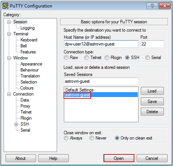
2.2. ISIS (UNIX) Processing Machine (astrovm-guest)

Open a PuTTY Session from the Windows Start Menu.
When the PuTTY Configuration window opens, select astrovm-guest under “Saved Sessions” to select it. Next, press “Open”. Enter the password when prompted. The password is the same for Windows and UNIX Guest Facility accounts.

Note that dpw-user#@astrovm-guest under “Host Name” will reflect the same two digits as at the end of the igswzawg…number on each machine.

#3. ISIS Machine and SOCET SET Workstation Interface for Guest Accounts

To transfer files between our ISIS processing machines and SOCET SET workstations, we use shared network drives. For our columnGuest Facility Users and participants of our training workshops, the shared network drive is named Z: on the SOCET SET Workstations. On ISIS machine astrovm-guest, this drive is accessed under /local_work.

Each Guest Facility account has access to localized folders and directories on the shared network drive based on the SOCET SET machine in use (these folders/directories are not accessible between SOCET SET workstations). When a Guest Facility user logs onto a SOCET SET machine or astrovm-guest, they will be automatically set to the root directory they have access to on the shared drive.

A SOCET SET project is divided into two folders: one to store data, the second to store images. The location of these folders is site dependent. At USGS Astrogeology, the project’s data folder is stored under D:/DATA and the project’s images folder is stored under E:/IMAGES. For any given project, SOCET SET will expect to find all data for the project in a folder path defined by D:\\DATA\\<ProjectName>, and all images in a folder path of E:\\IMAGES\\<ProjectName>.

Files will be transferred between the local D:\\DATA\\<ProjectName> and E:\\IMAGES\\<ProjectName> folders on the SOCET SET workstations, and the folders on the shared network drive Z:.

#4. ISIS Pre-Processing Overview In this section, we describe step-by-step procedures that are executed within ISIS as outlined in the Primer. This ISIS section focuses on ingestion of planetary image data and supporting geometric information for transfer to SOCET SET.

Note: Until ISIS has the calibration and “balancing” software to produce balanced cubes from PDS images, our procedure starts with the balanced cubes produced by the HiRISE Team. Note that balanced cubes are only available to HiRISE Team members.

For Guest Facility Users only. We will download the balanced cubes for your project before your arrival. Please contact us at [email protected] with the HiRISE stereo pairs you plan to process well in advance of your scheduled arrival date.

4.1. Create a working directory

Create a working directory on your ISIS machine for image processing. It is recommended that the working directory be named to represent the project/area you are working on. We will refer to the working directory as <ProjectName> from this point on in this tutorial. The UNIX command to create the directory is:

mkdir <ProjectName>

Note: The < and > characters surrounding ProjectName is syntax for a variable name and not part of the command.

4.2. Create image subdirectories

Under <ProjectName>, create separate directories for each imageto process (<imgdir>). We suggest that <imgdir> be the image name, e.g., PSP_001714_1415. UNIX commands are:

$ cd <ProjectName>
$ mkdir <imgdir1>
$ mkdir <imgdir2>

4.3. Download the images

NOTE: This requires special permission and an account on PIRL.

Download the RED balanced cubes (*RED*.balance.cub) into each < ProjectName/<imgdir> directory, as in the following examples.

$ cd <ProjectName><imgdir>`

rsync balanced cubes as follows:

$ rsync -rltvz hisync.lpl.arizona.edu::hirise_data/HiStitch/ESP/<ORB_dir>/<ESP_dir>/\*RED*\.cub

rysnc color cubes as follows:

$ rsync -rltvz hisync.lpl.arizona.edu::hirise_data/HiColorNorm/ESP/<ORB_dir>/<ESP_dir>/\*COLOR*\.cub

4.4. Image Quality Evaluation

Use the ISIS program qview to display the cubes before processing, and examine their quality. This step is intended to make sure the images do not have any signal-to-noise/haze problems (see Figure 1) that will make them undesirable for automatic DEM extraction. Steps are:

Activate the graphics viewing utility for the UNIX environment. For the Guest Facility accounts, activate the Xming utility from the tool bar.
Initiate the current ISIS release as follows:
```
$ setisis isis3
```
Then enter the qview command as follows:
```
$ qview <image_id>.balance.cub
```

Figure 1. Examples of noise and haze that may cause matcher problems

4.5. High Frequency Jitter Evaluation

Until correcting for spacecraft jitter is part of the HiRISE processing pipeline at U of A, check for extreme spacecraft jitter before continuing on, by running ISIS program hijitreg on the RED4 and RED5 CCDs as follows:

> setisis isis3
> hijitreg from=<RED4_balanced_cub> match=<RED5_balanced_cub> flatfile=<output\_flat\_file>

Once we have the flatfile in place, the following steps can be executed to check for jitter:

Bring <output\_flat\_file> into MS EXCEL
Calculate the difference of RegLine-FromLine
*Make a plot of the differences. *

The relative oscillation of the RegLine-FromLine difference gives an indication of the jitter in pixels, as shown in Figure 2.

Figure 2. hijitreg flat file imported into excel, and Regline -Fromline calculated (see the red field)

Evaluate the relative magnitude of the plot– not the absolute value of RegLine-FromLine, to determine the amount of jitter. Jitter that is less than 2 pixels is very workable, as in the example shown in Figure 3.

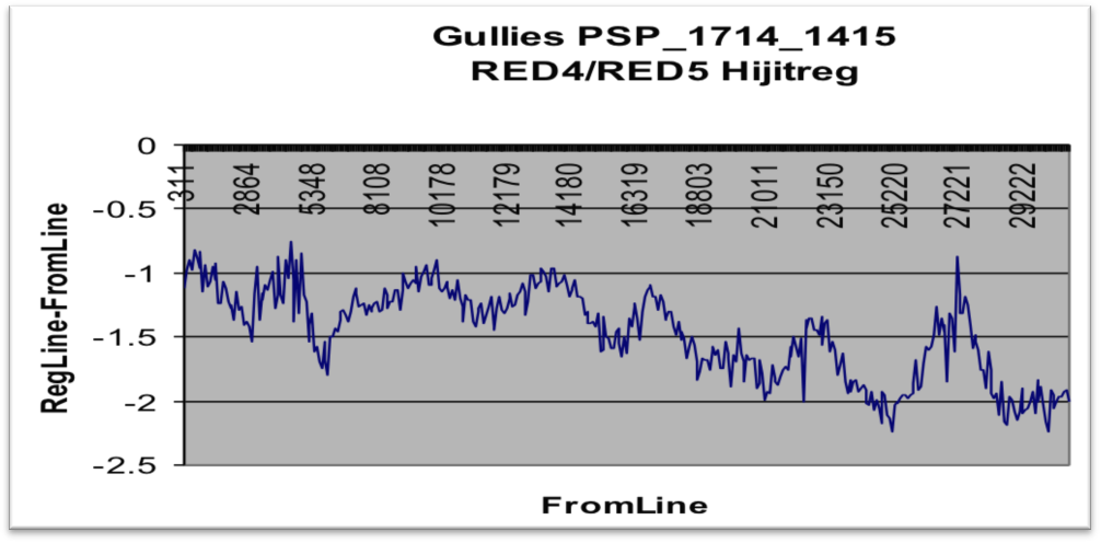Figure 3. Example plot of acceptable jitter.

If the overall jitter is between 2 - 3 pixels, you may have problems. At 4 pixels, you will definitely have problems.

If the jitter and image quality are acceptable, create a listing of RED.balance.cub files in <ProjectName>/<imgdir> and then run hi4socet.pl (details below). hi4socet.pl performs ISIS3 processing on HiRISE RED CCDs to generate a *.raw and a *_keywords.lis file for transfer to your SOCET SET workstation. Specifically, hi4socet.pl:

creates a 32-bit noproj'ed mosaic of the CCDs
converts the 32-bit mosaic to 8-bit and reports the stretch pairs used for the conversion to *_STRETCH_PAIRS.lis
converts the 8-bit image to a raw file (*.raw)
creates a list file of the SOCET SET USGSAstroLineScanner sensor model's keywords and values (*_keywords.lis)

Tip: Please try to organize your time as running hi4socet.pl may take hours to run.

4.6. Create image import list

hi4socet.pl requires the image cub list as input. Commands to generate this list are:

> cd <ProjectName>/<imgdir>
> ls \*.cub > cube_list

4.7. Process images for import

Commands to run hi4socet.pl are:

> setisis isis3
> hi4socet.pl cube\_list

4.8. Collect stereo statistics, MOLA DTM and MOLA track points

For HiRISE stereo processing in SOCET SET, we work in the Geographic Coordinate system. For input parameters to a project in geographic coordinates, you will need a planetographic latitude and positive east longitude reference point, and an estimated elevation range expected in the map area. Additionally, to control a stereo pair to MOLA, you will need the portion of the MOLA gridded data and MOLA Track data that cover the project area. These datasets must also be in the planetoographic latitude and positive East longitude system.

Based on the stereo coverage on a HiRISE (or MRO CTX) stereo pair, PERL script hidata4socet.pl will run ISIS3 and PEDR programs to generate the needed MOLA DEM and MOLA track files, along with a statistics files needed for the creation of <ProjectName> in SOCET SET. Simply run hidata4socet.pl within working directory <ProjectName> as follows:

> cd <ProjectName>
>hidata4socet.pl <ProjectName> <imgdir1>/<noproj_img1> <imgdir2>/<noproj_img2>

Where:

ProjectName = Name of the SOCET SET project
<imgdir1>/<noproj\_img1> = First noproj'ed image of a stereo pair
<imgdir2>/<noproj\_img2> = Second noproj'ed image of a stereo pair

The output products of hidata4socetl.pl are as follows:

A MOLA DEM as an ISIS3 cube and an ascii ARC Grid. The MOLA DEM will be stored in <ProjectName>/MOLA_DEM and named <ProjectName>_mola.cub and <ProjectName>_mola.asc.
The MOLA track data as a Shapefile and a table file. The track data will be stored in <ProjectName>/MOLA_TRACKS. Shapefile will be named <ProjectName>Z.shp. The table file will be named <ProjectName>.tab. (Other miscellaneous files will also be stored in <ProjectName>/MOLA_TRACKS, but are not directly used in the stereo processing.)
A file listing the geographic reference point coordinate and elevation range of the stereo-overlap area. This file will be named <ProjectName>_SS_statistics.lis, and located in <ProjectName>.

#5. SOCET SET Workstation Setup

5.1. SOCET SET root paths

There are three primary paths defined in the SOCET SET defaultconfiguration. These paths are site dependent, and are:

*<install\_path> = The path for executables and system level support files in the SOCET SET application suite. At the Astrogeology Guest Facility, this path is C:\SOCET_SET_5.6.0.

*<data\_path> = The default root path to the various project folders and project files (*.prj). At the Astrogeology Guest Facility, this path is D:\DATA.

*<image\_path> = The default root path to imagery for various project folders. At the Astrogeology Guest Facility, this path is E:\IMAGE.

In the case of a project named<ProjectName>, SOCET SET will expect to find all images in a folder path of<image\_path>\<ProjectName> (e.g., E:\\IMAGES\\<ProjectName>), and all data for the project in a folder path defined by<data\path><ProjectName> (e.g., D:\\DATA\\ProjectName>).

5.2. Planer Stereo Display Calibration

In order to see 3D (stereo) correctly, it is important to have the two screens meet the beam splitter display device at sympathetic angles; this is accomplished by adjusting the beam splitter set screws to change the orientation of the beam splitter relative to the two display monitors. If the display appears “de-focused” it is necessary to make these adjustments before the measurement process is begun, in order to reduce the eye strain associated with the stereo viewing process.

5.3. Starting SOCET SET

The very first step is to locate the following icon on the Windows Desktop. Double click on this icon to start SOCET SET, and wait until all components are activated.

5.4. Status Message Window

The Status Message Window should come up automatically (usually in the lower left corner of the console monitor.) This window captures status messages and error messages issued by SOCET SET, and is helpful to have open at all times.

If the Status Message window did not come up, do the following:

From the SOCET SET menu bar, select Tools > Status Message.

6. Create a SOCET SET Project

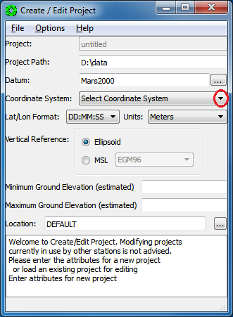
For HiRISE stereo processing, create a project in Geographic Coordinates, using Mars2000 as the datum. (Note that SOCET SET also allows a project in a map projection. This would generally be needed only if the project is (a) polar and (b) spans a large range of latitudes.)

6.1. Launch the Project Editor

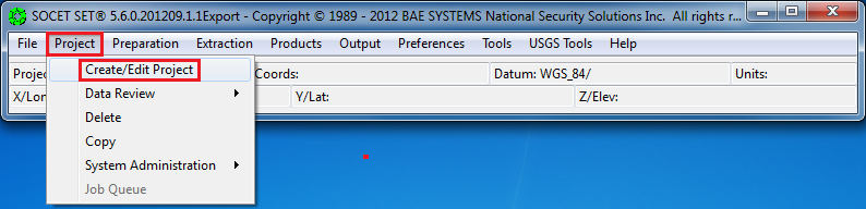
From the SOCET SET menu bar, select “Project” > “Create/Edit Project”.

6.2. Create a new project

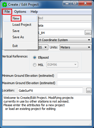
Select “File” > “New”

6.3. Set the Datum

Press the box next to the datum field to bring up the “Select a Datum” window.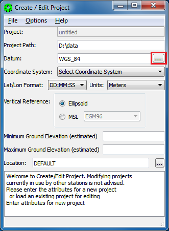
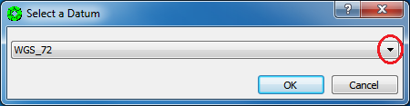
Right-Click on the down arrow in the selection window to display drop-down box of options.
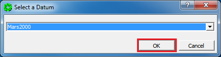
Scroll about 90% down the list, or press the letter M to skip down the list to the datums starting with the letter M. Select Mars2000 and then press OK.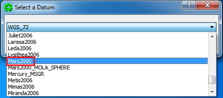

6.4. Set the Coordinate System

For SOCET SET projects in Geographic Coordinates, you must enter a reference latitude and longitude coordinate (this is equivalent to the center longitude and center latitude of the equi-rectangular map projection.)

The reference latitude and longitude coordinates can be found in the SOCET SET project statistics file, generated by hidata4socet.pl.

Use a text editor to open <ProjectName>_SS_statistics.lis. For columnGuest Facility Users, this file is located in Z:\\<ProjectName> and named <ProjectName>_SS_statistics.lis.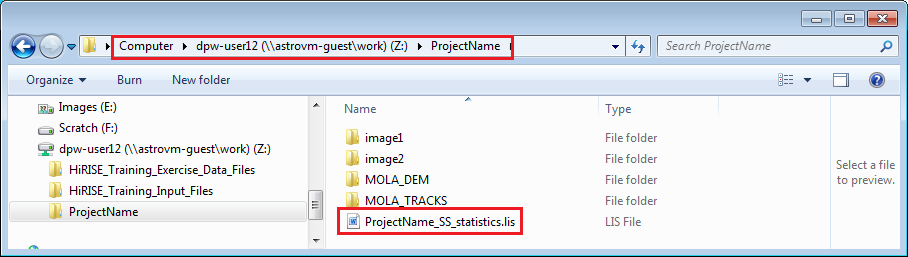
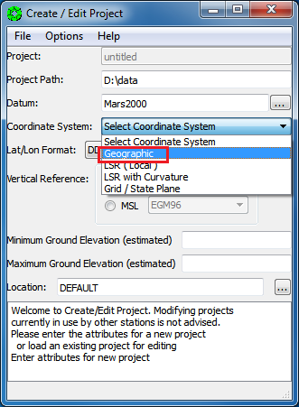
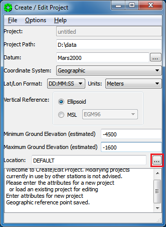
On the Create/Edit Project window, Left-Click on the down arrow next to Coordinate System name to display drop-down box of options and select Geographic.
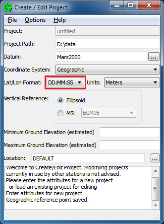
You will be prompted to enter a reference point within the project in Degrees Minutes Seconds (DMS) format. Enter the coordinate listed in <ProjectName>_SS_statistics.lis file generated by hidata4socet.pl. Then press OK.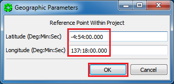
Do not close <ProjectName>_SS_statistics.lis yet. It is needed again, below.
Keep the default Lat/Lon Format definition: DD:MM:SS

Note: We’ve tried using a lat/lon format of decimal degrees, but found in some cases the lat/lon format is in DMS regardless. So we are sticking with DMS throughout SOCET SET processing.
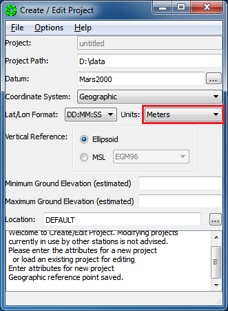
Keep the default Units definition: Meters

6.5. Select a vertical reference

Press the Ellipsoid radio button (this should be the default).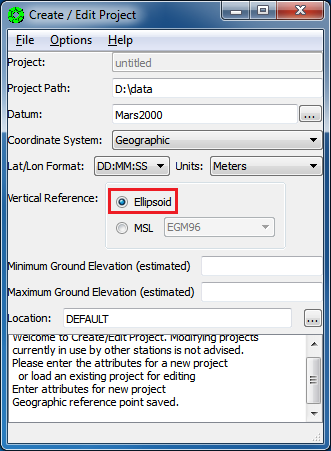
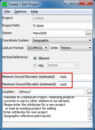
For the Min and Max Ground Elevations, enter the minimum and maximum elevations listed in the project statistics file generated by hidata4socet.pl <ProjectName>_SS_statistics.lis.

Note: A rough estimate of the expected elevation range over the project area is all that is needed.
Now close <ProjectName>_SS_statistics.lis.

6.6. Define the location of the images folder/directory

Press the box next to the Location field to bring up a selection window.
Press Edit Locations to add a directory/folder to the File Location list.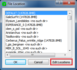
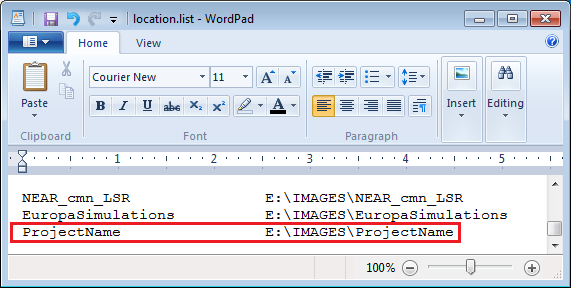
The WordPad editor will be initiated. Scroll to the bottom of the file. Enter your desired location/folder name following the format of the location.list file, then save and exit from WordPad.

Note: (1) Do not use tab in editing the File locations information as it will lead to errors in intrepretation by SOCET SET. (2) We scroll to the bottom of the list because the top three lines define a default images folder, and the default should not be changed.
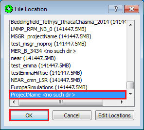
From the File Location window (it remained open while editing the location.list file), you can now scroll to the bottom of the list and select your location/folder for the project to store and create images in.

Note: If your folder name is not listed, press Cancel and reopen the file (by pressing the box next to Location field) to see your folder name.

Note: Upon data entry the window may report that there is “no such directory”, it is safe to ignore this prompt and continue. (The directory will be created for you once project creation is complete.)

6.7. Create the Project Files and Folders

Select File > Save As.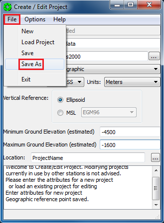
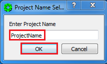
Enter the name of the project in the pop-up window, then press “OK”.

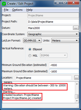
If the images folder did not previously exist (set in the previous section), SOCET SET will now create it, along with the data folder. For an elevation range below -300 meters, or greater than 10000 meters, you will get a warning message. This warning can be ignored for non-Earth projects.
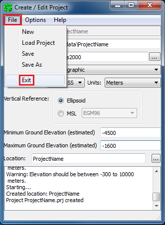
Select File > Exit.

#7. Load Project

From the SOCET SET menu bar, select File > Load Project.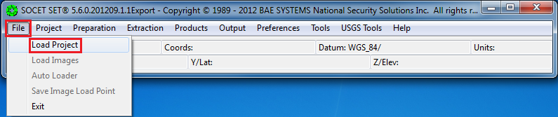
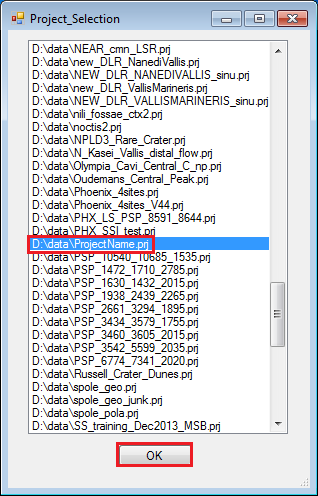
From the pop-up window, scroll to find your project (the list of projects is in alphabetical order), select it and press OK.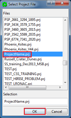

#8. Transfer Files to SOCET SET Workstation

From the ISIS processing machine, we need the following files generated by the hi4socet.pl and hidata4socet.pl scripts for each image in the ISIS pre-processing stage:

<ProjectName>/<imgdir>/<noproj_img>/*.raw: The distortion corrected images in 8-bit raw format
<ProjectName>/<imgdir>/<noproj_img>/*_keywords.lis: The associated SOCET SET USGSAstroLineScanner keywords files, and
<ProjectName>/<imgdir>/<noproj_img>/campt*.prt: The campt report associated with the image.

If your plans are to control the stereo pair to MOLA, you will also need the following files generated by the hidata4socet.pl script in the ISIS pre-processing stage:

<ProjectName>/MOLA_DTM/*.asc: The MOLA DTM as an ARC Grid.
<ProjectName>/MOLA_TRACKS: The entire MOLA Tracks directory which contains the files associated with the Shape file.

It is strongly recommended that the *.raw, *keywords.lis and campt*.prt files (items 1, 2 and 3 from the above list) be copied into a subfolder named ISIS in the project’s images folder on the SOCET SET machine (e.g., E:\\IMAGES\\<ProjectName>\\ISIS), and the MOLA data files (items 4 and 5, above) be copied into the project’s data folder (e.g., D:\\DATA\\<ProjectName>).

8.1. File Transfer for Guest Facility Users

8.1.1. Create ISIS subfolder

Bring up Windows Explorer and navigate to E:\\IMAGES\\<ProjectName>.
Create a folder in E:\\IMAGES\\<ProjectName> and name it ISIS.

8.1.2. Transfer Images and Keywords Files

Navigate into E:\\IMAGES\\<ProjectName>\\ISIS.
Open a second Windows Explorer window, and navigate into Z:\\<ProjectName>\\<image>.
Copy the campt_<image>.prt, <image>.raw and <image>_keywords.lis files into E:\\<ProjectName>\\ISIS. Repeat for all images processed in Z:\\<ProjectName>.
Note that there are no subfolders under E:\\<ProjectName>\\ISIS.

8.1.3. Transfer MOLA Data

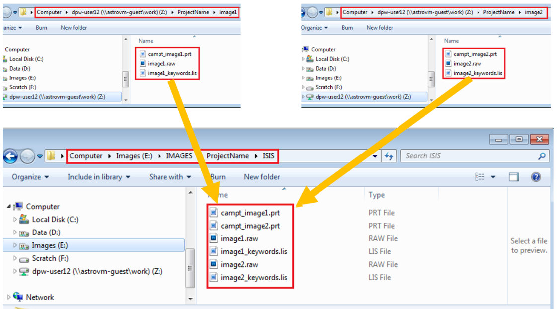
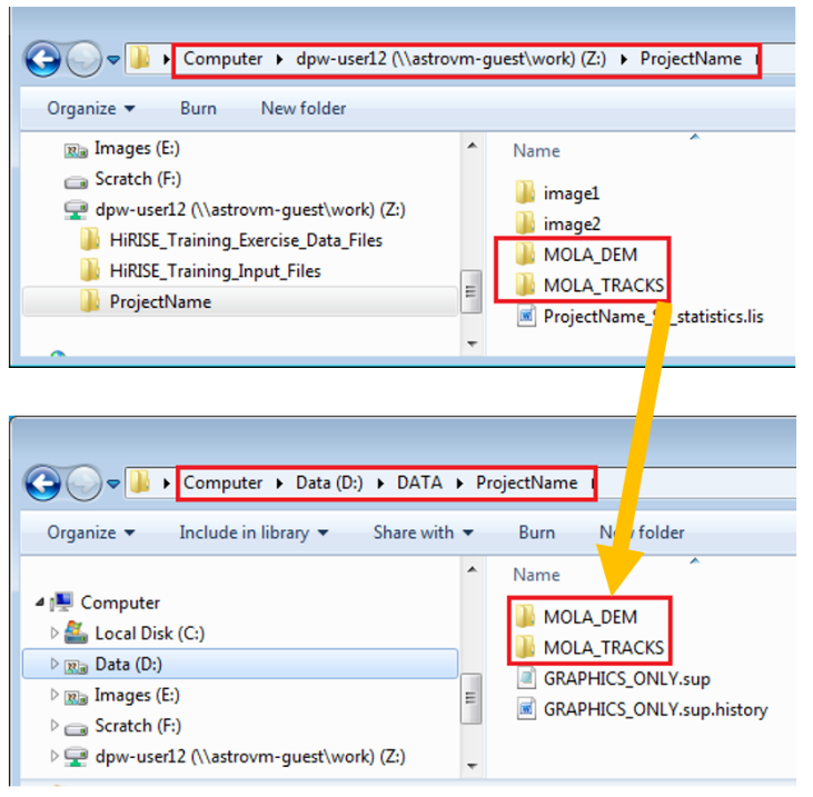
Navigate into D:\\DATA\\<ProjectName>.
Open a second Windows Explorer window, and navigate into Z:\\<ProjectName>.
Copy the MOLA_DEM and MOLA_TRACKS folders from Z:\\<ProjectName> into D:\\DATA\\<ProjectName>.

9. Import Pushbroom/Linescanner Images

Select USGS Tools > Imports > Import Pushbroom.
From the USGS Import Pushbroom window, if the project listed is your current project confirm the Project by clicking the Project File checkbox. Otherwise press Project File… to bring up the Project_Selection window, select the current project, and press OK.
Press Image Path… and navigate to the project’s E:\\IMAGES/<ProjectName>/ISIS folder. Then press OK.

Note: The ISIS folder MUST contain the <image>_keyword.lis and <image>.raw files.

![](media/image42.png)

Either select Individually the images required for the project or use the Select All button to import all the images in the list.
Press Execute, and the utility will populate then execute program import_pushbroom to build the required images and project support files.

Note: This utility expects that the image name and the keywords file are in agreement with each other, with _keyword appended to the base file name. For example, An Image file named Image_123.raw should have an associated keywords file of Image_123_keyword.lis.

If your import fails then please verify that the naming convention is correct.
Close the Command Prompt Window when import is complete for all images selected.

#10. Load Images

From the SOCET SET menu bar, select File > Load Images.
Select a Left and Right Image to display in the stereo monitor by clicking on the image id in the Left and Right panels. (Selected images will be highlighted.)

Note:
1. For image display, it does not matter which image you choose for the left or right “eye”. SOCET SET will align the images for best stereo viewing regardless of the order selected, however, you will notice a 180 degree rotation of the stereo pair depending on the order you select the images.
1. The Refresh button only refreshes the list of images, it does not actually reload images. Press the “Refresh” button if there are newly created images not showing up on the list.
Under View Control Panel settings: Ensure that View = 1 and that Load Point is selected.
Press Load.
Press Close

11. Establish Stereo Display Settings

11.1. View 1 Window Settings

Below is an example of the settings typically used for View 1, and may vary depending on system and data uniqueness. These settings are to be established on the View 1 window (the stereo display monitor).

11.2. Tracking Sensitivity

Tracking sensitivity controls the movement and speed of the TopoMouse (i.e., extraction cursor.) Before proceeding, please check that the tracking sensitivity is correct for the TopoMouse (details below.)

Also, if SOCET SET crashes, the tracking sensitivity values are typically lost, and the TopoMouse behaves poorly. When this happens, you must reset the values.

From the SOCET SET menu bar, select Preferences > Tracking Sensitivity.
In the diagonal of the upper matrix, enter 0.1, 0.1, **-**0.1 for X, Y and Z motion, respectively, and zeros everywhere else. Then press Close. Note that the Z motion is a negative value.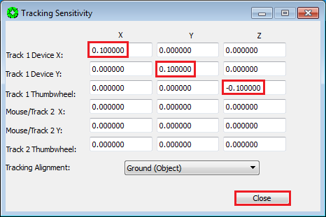
Press Yes on the pop-up window to save the new values for future sessions.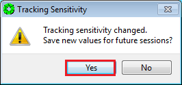

12. Import MOLA ArcGrid DTM

From the SOCET SET menu bar, select Preparation > Import > Terrain > ArcGrid.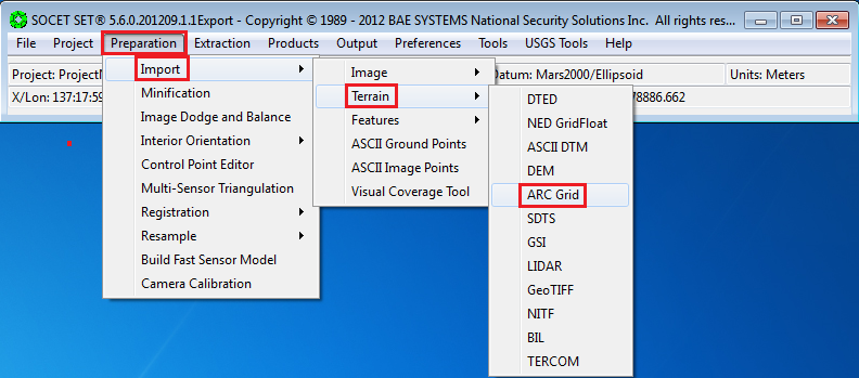
Press the button next to the Input ASCII ARC GRID File field to bring up a file selection window.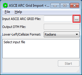
Navigate to D:\\DATA\\<ProjectName>\\MOLA_DEM. Select <ProjectName>_mola.asc, and press Open.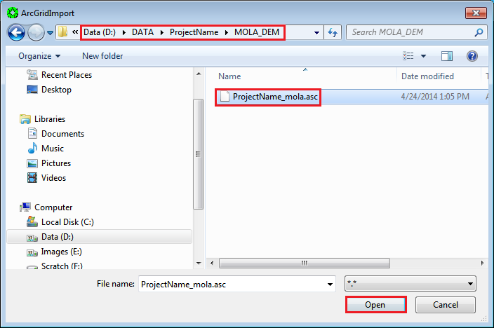
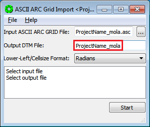
Enter output DTM File name.

The easiest way is to copy/paste the input name without the .asc extension.

Then press the return key and SOCET SET will automatically add the path and dth extension.
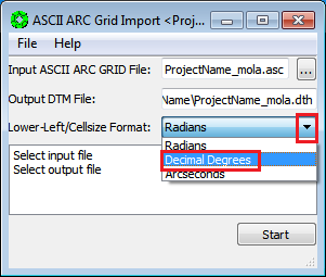
Set the Cell size Format to Decimal Degrees. Right-Click on down arrow to display drop-down box of options and select Decimal Degrees.
Press Start to import the MOLA ARC Grid.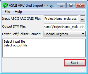
Select File > Exit when import is finished.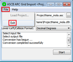

12.1. Verify MOLA DTM Import

Display the MOLA DTM as contours using Interactive Terrain Edit (ITE) to verify the import.

From the SOCET SET menu bar, select Extraction > Terrain > Interactive Edit.
Select File > Open DTM… on the ITE window.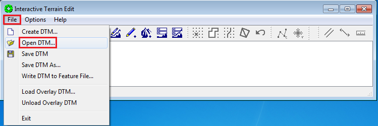
Select <ProjectName>_mola and press OK.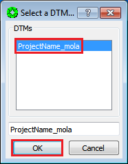
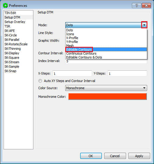
Press the Setup DTM Graphics icon on the ITE window.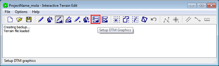
On the Preferences window, Left-Click on down arrow next to the Mode field to display drop-down box of options, and select Editable Contours.
Set the Contour Interval field to 50.0, and press OK.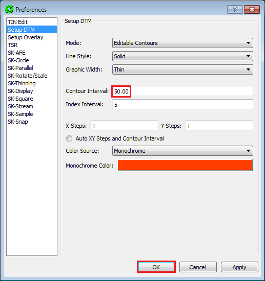
Press the Draw Terrain Graphics icon on the ITE window. The MOLA contours will be drawn on the View 1 (stereo display).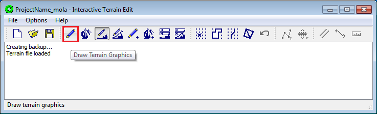
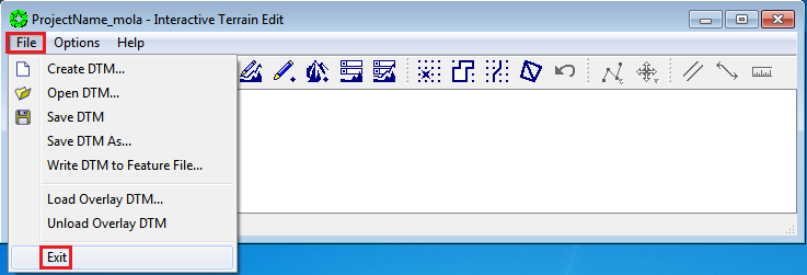
When the MOLA Grid import is verified, select File > Exit on the ITE window.

13. Import MOLA TRACKS Shapefile

From the SOCET SET menu bar, select Preparation > Import > Features > Shapefile.
Select File > Open Shapefiles… in the Shapefile Import window.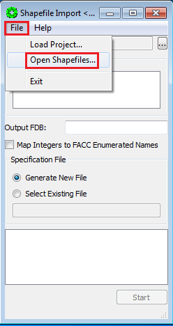
Navigate to D:\\DATA\\<ProjectName>\\MOLA\_TRACKS. Select <ProjectName>Z.shp, and press Open.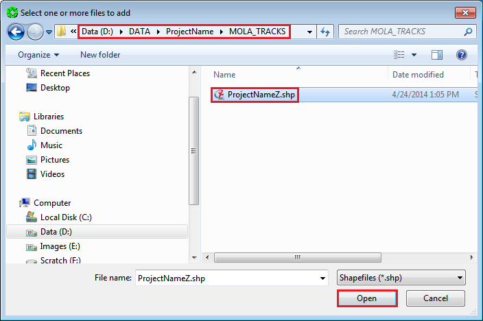
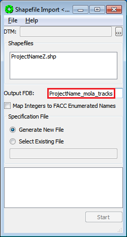
Enter the Output FDB name without an extension. Then press the enter key and SOCET SET will add the project data path and file extension.
Turn on radio button for Generate New File, and press Start to import the MOLA Track Points.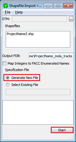
Select File > Exit when import is finished.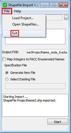

13.1. Verify MOLA Track Import

Display the MOLA Track points using Feature Extraction (FE) to verify the import.

From the SOCET SET menu bar, select Extraction > Feature > Feature Extraction.
Select File > Open FDB…` in the FE window.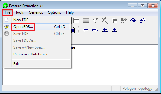
Select <ProjectName>_mola_tracks, then press OK.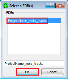
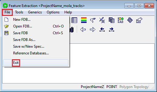
The Feature Extraction tool should have defaulted to Auto Draw On, and the Tracks should be drawn on View 1. If not, press the Draw icon to draw the Tracks.
When the MOLA Track import is verified, select File > Exit on the FE window.

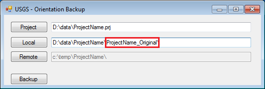
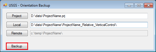
14. Backup Original Image Support Files

Before beginning the image control procedure, store a copy of the original (a-priori) support files in a subfolder of the project’s data folder named <ProjectName>_Original. Throughout the control procedure, we will copy the contents of this subfolder back into the project’s data folder for a clean adjustment, or to reset the support files if an adjustment diverges.

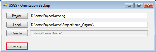
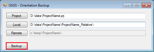
From the SOCET SET menu bar, select USGS Tools > Backup Orientation.
Make sure the current project name is listed in the Project field. If not, press “Project” to select the current project, then press “OK”. (Otherwise the backup will be made in, and for, the wrong project!)
Replace Backup_0 with _Original in the Local folder name field.
Press Backup.

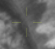
15. Setup of Extraction Cursor For Beginners

Experienced operators will normally use a very small dot for their extraction cursor (also known as a floating mark), but this type of floating mark will usually prove to cause eye fatigue and pointing errors for novice operators. The following is a recommendation only and not crucial to stereo processing.

From the SOCET SET menu bar, select Preferences > Cursor/Graticle Editor.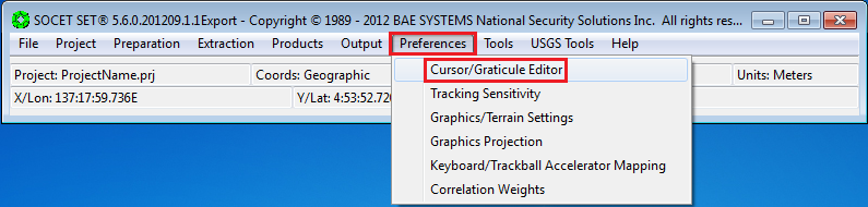
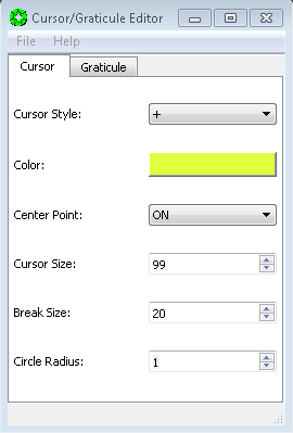
The following window will become active.
The following recommended settings will yield the cursor shown below:

Cursor Style	Cross
Color	Yellow, or a Color Highly Visible on BW image
Center Point	On
Cursor Size	99
Break Size	20
Circle Radius	1

Select File > Exit on the Cursor/Graticule Editor window.

#16. Determine Nadir-Most Image for Image Control

During the Relative Orientation and Vertical Adjustment to MOLA image control stages, we will hold the nadir-most image. To determine which is the nadir most, use a text editor to open the campt_<image>.prt files in E:/IMAGES/<ProjectName>/ISIS, and make note of the image with the smallest Emission Angle.

#17. Image Control Overview and Naming Convention

Controlling HiRISE images to MOLA Tracks is a three-stage approach. Stage 1 is a Relative Orientation to remove y-parallax between the images of the stereo pair which aids stereo viewing. Stage 2 is Vertical Adjustment of the stereo model to align it in height (elevation) to the MOLA surface; which aids viewing the MOLA DTM or MOLA Tracks superimposed over the stereo pair. Stage 3 is an Absolute Orientation to align the stereo model with the MOLA Tracks, if-and-only-if there are sufficient MOLA Track data to accomplish the orientation. Depending on the analyst’s desired level of accuracy, the Image Control process can stop at any of the three stages.

We ask that all users follow the same naming convention for triangulation file names and backup folder names (listed below). Following the same convention allows for ease of transition with multiple users accessing a project.

Triangulation files (*.atf) will be named as follows:

<ProjectName>_Relative.at – Relative Orientation
<ProjectName>_Rel_VertCtrl.atf – Vertical Adjustment using relative orientation image parameters and vertical (Z) control points.
<ProjectName>_Abs_XYZ_Ctrl.atf – Absolute Orientation using absolute orientation image parameters, and XYZ Control.

Project Backup Folders will be named as follows:

<ProjectName>_Original – Stores the original (a-priori) image support files.
<ProjectName>_Relative – Stores the result of the Relative Orientation
<ProjectName>_Relative_VerticalControl – Stores the result of the Vertical Adjustment
<ProjectName>_ Absolute_XYZ_Control – Stores the result of the Absolute Orientation

#18. Image Control Stage 1 - Relative Orientation

In the Relative Orientation stage we will remove the Y-parallax between the stereo images. Y-parallax is separation of the stereo images in the Y (up-and-down) direction.

##18.1. Multi-Sensor Triangulation Setup

From the SOCET SET menu bar, select Preparation > Multi-Sensor Triangulation.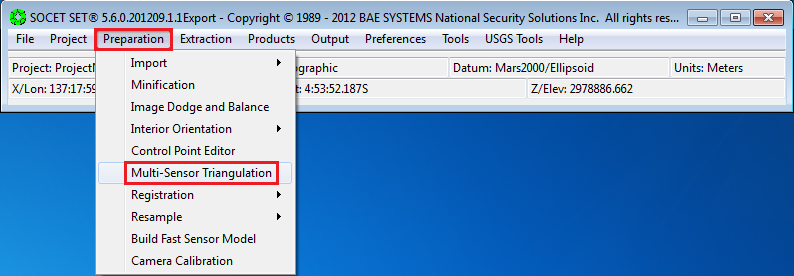
Press the box next to the Triangulation file field to bring up a file selection window.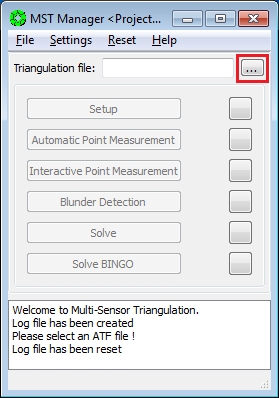
Enter <ProjectName>_Relative as the name of triangulation file and press Save.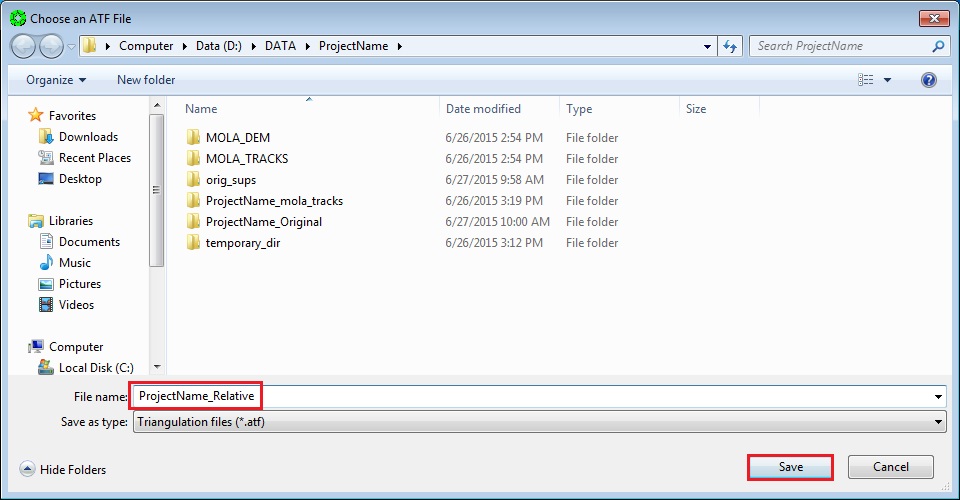
Press Setup.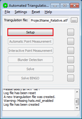
In the Setup window, press Add.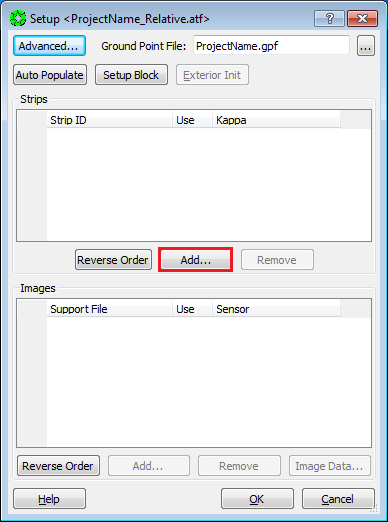

Note that in the Setup Window, the Ground Point File: (to be created) will automatically be named after the project name.
In the Strip ID Sequence box, use the default value of 1, and press OK.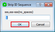
You will be prompted to Select Support Files. Do this by highlighting each image in the Available list and moving them to Selected list via the arrow buttons. Press OK when done.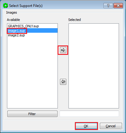
The selected images are now listed in the Setup window. Select the nadir-most image, and press Image Data….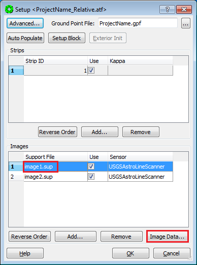
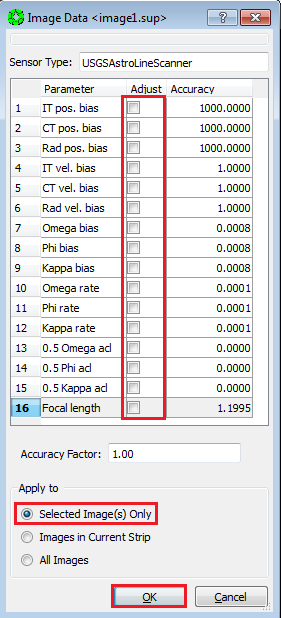
In the Image Data window:

a. make sure no check boxes are checked in the Adjust field.

b. Turn on radio button Selected Image(s) Only in the Apply To section.

c. Press “OK”.

Note:
1. Not allowing any parameters to adjust holds this image to it’s a-priori position and pointing.
1. Please ignore the values listed in the Accuracy field, as they may not be applicable to the setup in certain cases
Go back to the Setup window. Select the Support file of the other image, and press Image Data….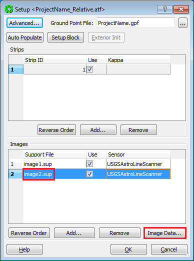
In the Image Data window:

a. Turn on the check boxes for the parameters listed below, and enter the corresponding accuracy values. (All other parameters are off. If a parameter is checked, it will be allowed to adjust. If it is not checked, it will remain unchanged when the triangulation is run.)

b. Turn on radio button Selected Image(s) Only in the Apply To section.

c. Press OK.

Parameter Accuracy

IT pos. bias 100 m

CT pos. bias 100 m

Radial pos. bias 10 m

IT vel. bias 13 m/s

CT vel. bias 13 m/s

Radial vel. bias 1.3 m/s

Kappa bias 0.1 degree
Press OK in the Setup window.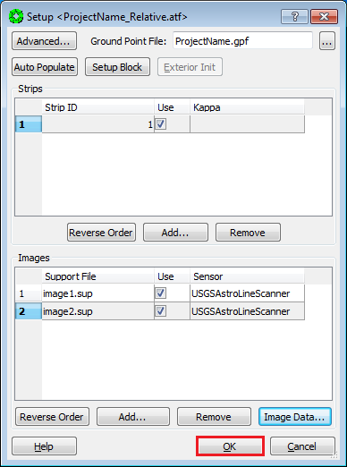
Select File > Save Triangulation File in the Automated Triangulation window.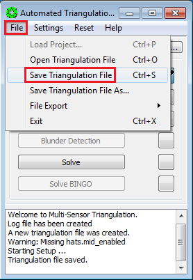

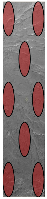
18.2. Tie Point Distribution

Using Interactive Point Measurement (details below), we will measure two “tie points” per region, as distributed in 8 regions shown here, for a minimum of 16 points. This point distribution is called “Buddy Points”, and aids in highlighting poor image measurements when solving a bundle adjustment.

NOTE: We want to convert as many of these tie-points to z-only control in the Vertical Adjustment to MOLA stage, so when possible avoid steep slopes areas.

18.3. Interactive Point Measurement Setup

Ensure that the View 1 window in the stereo display is set for stereo mode.
Be seated squarely in front of the stereo display (with stereo viewing glasses).
Press Interactive Point Measurement from the Automated Triangulation window.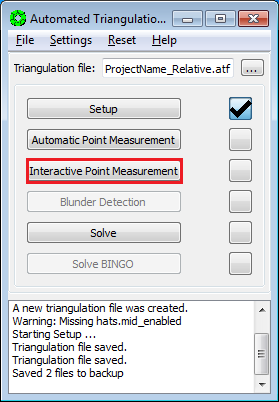
Press Settings in the Interactive Point Measurement (IPM) window.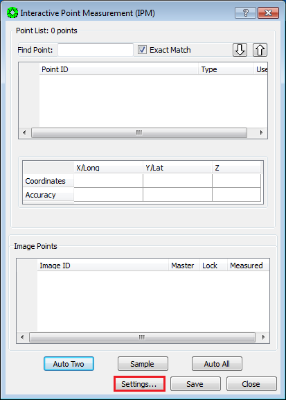
In the Settings for IPM window, check the Auto Img List box, then press “Close”.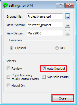

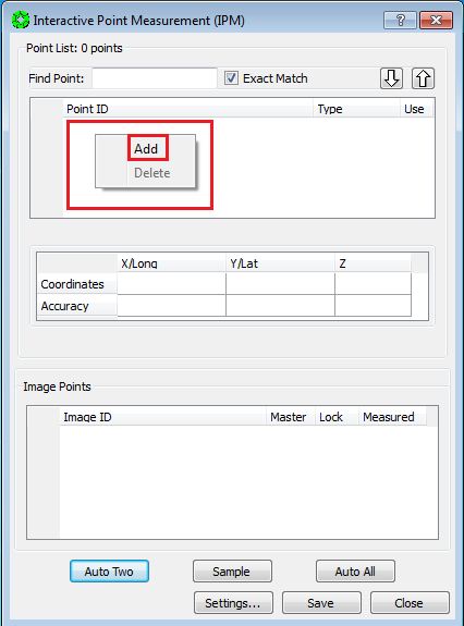
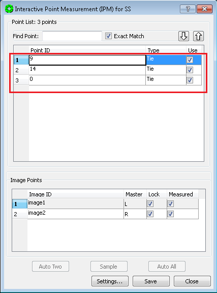
18.4. Manual Tie Point Measurement

In the IPM window:

a. Right Click in the Point ID field.

b. Select “Add” in the pop-up window.
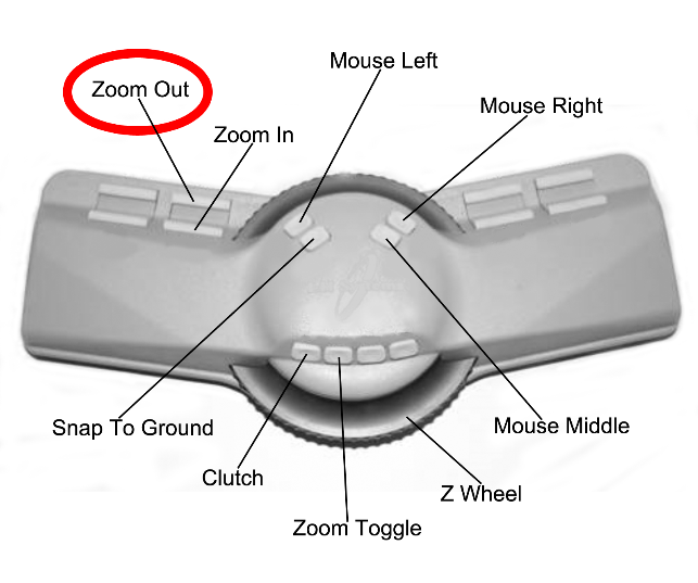
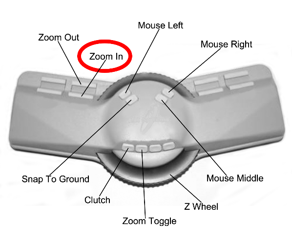
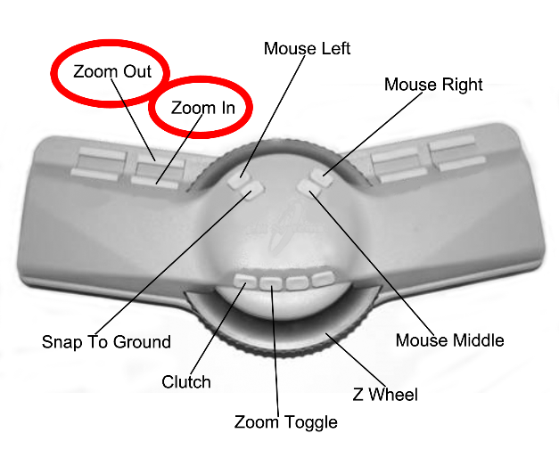
On the TopoMouse, use the zoom out button (repeatedly), to view full extents of the stereo model.
Move cursor to first (or next) region for tie point measurement.
Use TopoMouse “Zoom in” button (repeatedly) to set view to approximately 8:1 ratio.
Locate an area where terrain is relatively continuous with minimal slope, and move extraction cursor to that location.
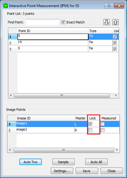
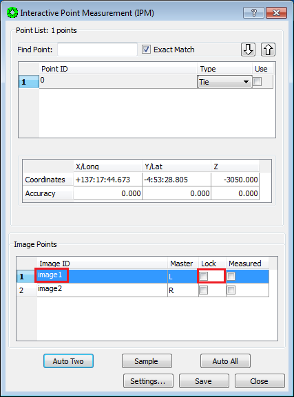
In the IPM window, lock the Left image by checking its Lock box.
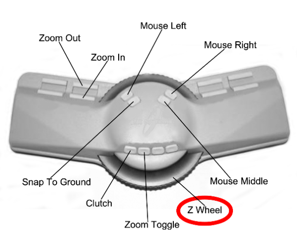
Clear parallax by moving the Right image only and place the extraction cursor on the ground. You may use the Z wheel to fine-tune the height adjustment of the extraction cursor after Y-parallax is removed.

Note: You need to practice the placement of the cursor on the ground several times, until you have clear sense of when it is above or below the ground. See Appendix: A-3 Placing Dot on the Ground.
Use the TopoMouse “Zoom In” button (repeatedly) to set view to 1:1 ratio.
In the IPM window, Unlock the Left image by unchecking its Lock box.
Refine the extraction cursor position to a highly discernible location that is representative of surrounding terrain and free of high relief or slope. Do not measure edges of shadows, because shadows “move” between image scenes, and the extraction cursor will not be truly on the ground.
In the IPM window, lock the Left image by checking its Lock box.
Refine the parallax removal (at ground level) by moving the Right image only. In other words, put the dot on the ground.

Note: Experienced analysts with good stereo acuity to recognize when auto-correlation has correlated to a false positive result, may want to use the “Auto-Two” feature in this step. For details, see Appendix: A6.1 Auto Two Feature in IPM.
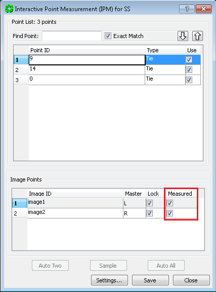
Press Sample on the IPM window to collect the point measurement.

Note: Sample stores the measurement in computer memory only. After Sample is pressed, both images will be locked and measured.
Press Save on the IPM window to write the measurement to disk.
Start measurement of second (buddy) point in the same region:

a. In the IPM window, Right Click in the Point ID field.

b. Select Add in the pop-up window.
Move the extraction cursor to a new location in the current field of view.
In the IPM window, lock the Left image by checking its Lock box.
Refine the parallax removal (at ground level) by moving the Right image only. In other words, put the dot on the ground.

Note: Experienced analysts with good stereo acuity to recognize when auto-correlation has correlated to a false positive result, may want to use the “Auto-Two” feature in this step. For details, see Appendix: A6.1 Auto Two Feature in IPM.
Press Sample on the IPM window to measure the (buddy) point.
Press Save on the IPM window to write the measurement to disk.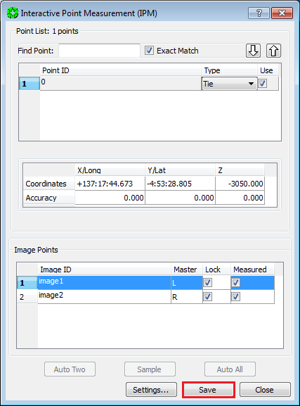
Go To: Step 1 of this section (17.4 Manual Tie Point Measurement), and repeat this procedure for each of the regions defined in 17.2 Tie Point Distribution.
After completing the measurement process for all 8 regions (16 points), press Close on the IPM window.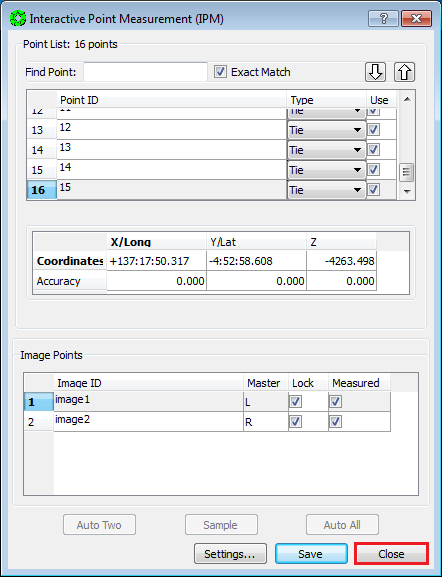

18.5. Bundle Adjustment

Return to the Automated Triangulation / Full Block menu in the MST, and activate the adjustment procedure by pressing Solve.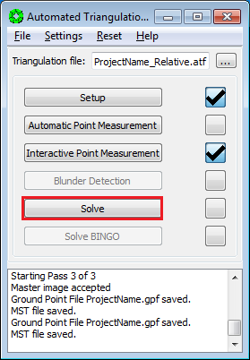
The Simultaneous Solve window will open, along with a Backup pop-up window. Press Yes on the pop-up to overwrite back up files.
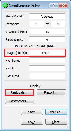
In the Simultaneous Solve window, press Start to perform the bundle adjustment.
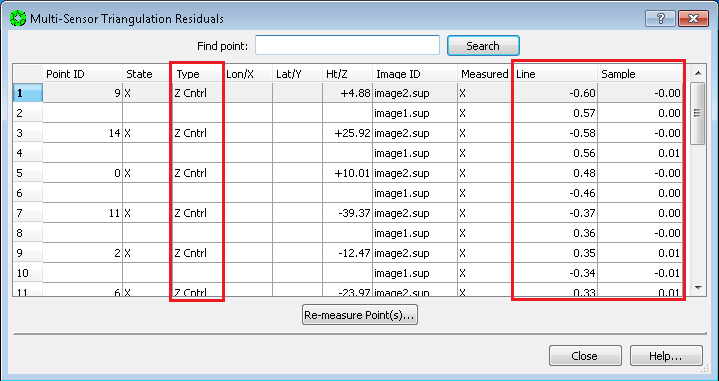
Once the adjustment is completed, the Simultaneous Solve window will be updated with a report of: Number of ground points generated, solution redundancy, and most importantly the RMS residual error (in Image pixels).

An acceptable solution has (1) an Image (pixels) RMS of ~0.6 or less, and (2) no individual point measurement has an error greater than 2 pixels.

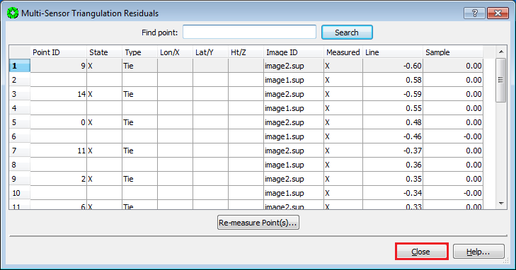
Press “Results” in the “Simultaneous Solve” window to review the error of individual point measurements.
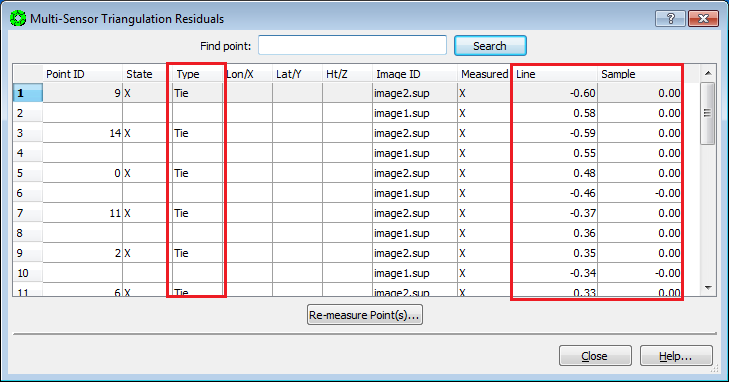
Points in the Residuals window are grouped by Type, and automatically sorted from highest to lowest residual. The Line and Sample fields list the point measurement errors in pixels. In a Relative Orientation, all points are Tie, so inspecting the top of the list will suffice.
If points have pixel errors greater than 2.0 pixels, SKIP TO: 17.6 Point Re-Measurement Process. Otherwise, continue to the next step.
If the image RMS is < ~0.6 pixels, and the maximum point measurement error is < 2.0 pixels, then press “Close” on the Multi-Sensor Triangulation Residuals window.
Press Save on the simultaneous solve window.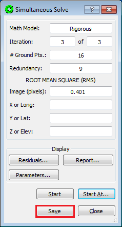
Press Yes on the Done pop-up window.
Press Close on the Simultaneous Solve window.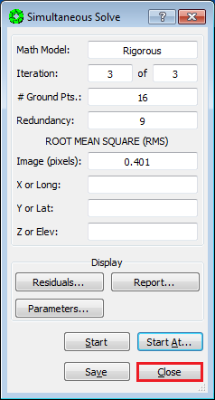
Select File > Exit on the Automatic Triangulation window.

Relative Orientation is now complete!
SKIP: 17.6 Point Re-Measurement Process, GO TO: 17.7 Re-Load Images.

18.6. Point Re-Measurement Process

Continuing from 17.5 Bundle Adjustment…

On the Multi-Sensor Triangulation Residuals window, Left-Click on the Point ID(s) of the points to re-measure. (Hold the Control Key down to select multiple points.) Then press Re-measure Point(s)…. The re-measure point window will now open with the points selected.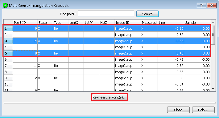
Left-Click on the point to re-measure. The View 1 (stereo display) will display the current point measurement.
You have an option of relocating the point or clearing parallax:

a. To relocate the point, Un-check the boxes in the Measured field for both images.

b. To remove residual parallax, Un-check the Measured box for the Right image only.

NOTE: Un-checking a Measured box will also un-Lock the image so it is free to move using the TopoMouse.
If you are re-locating the point, place the extraction cursor on the feature in the Left image that you would like to measure. Then Lock the Left image by checking the box in the Lock field for the Left image.
For either option (re-locating the point, or removing residual parallax), clear the parallax by moving the Right image only (i.e., put the dot on the ground).
Press Sample to collect the point measurement.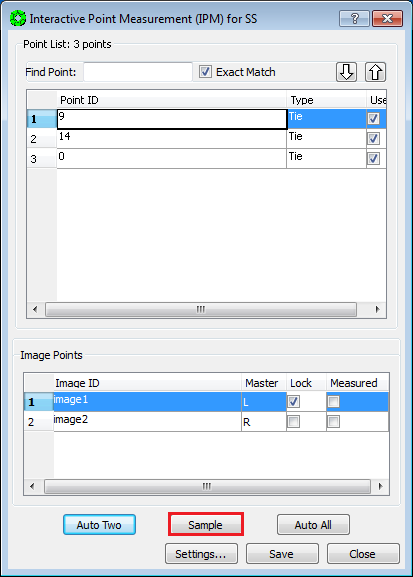
Press Save to write the measurement to disk.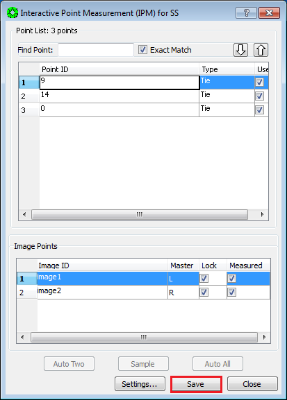
Repeat re-measurement process for remaining points in the list. (Go back to step 2.)
Press Close after all points in the list are re-measured.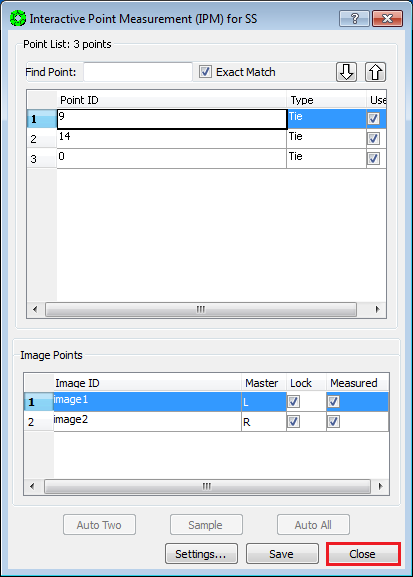
Press Close on the Multi-Sensor Triangulation Residuals window.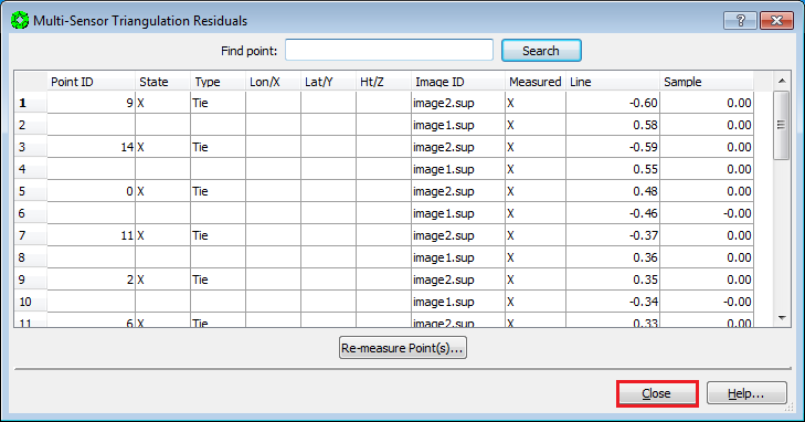
Press Start on the Simultaneous Solve window.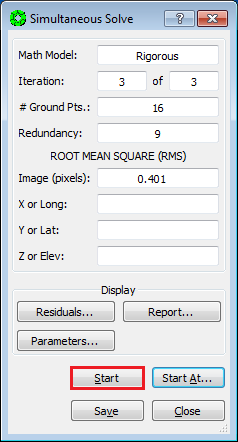
Press Residuals on the Simultaneous Solve window and make sure no individual point has an error greater than 2 pixels.
If there are points with larger than 2 pixel errors, Go To: Step 1 of this section (17.6 Point Re-Measurement Process) and further refine the measurements.
If the overall RMS < ~0.6 pixels, and all points have less than a 2 pixel error, we will exit Multi-Sensor Triangulation, and re-enter it in order to refresh the values stored in computer memory. First press Close on the Multi-Sensor Triangulation Residuals window.
Press Close on the Simultaneous Solve window. (Do Not Press Save.)
Press No to Saving Files in the Done pop-up window.
Select File > Exit on the Automatic Triangulation window.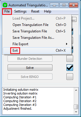
From the SOCET SET menu bar, select Preparation > Multi-Sensor Triangulation.
Press Solve on the Automatic Triangulation window. (The triangulation file, ProjectName_Relative, should load automatically.)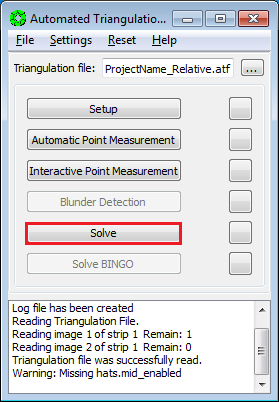
Press Yes on the pop-up to overwrite back up files.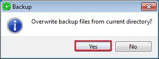
Press Start on the Simultaneous Solve window.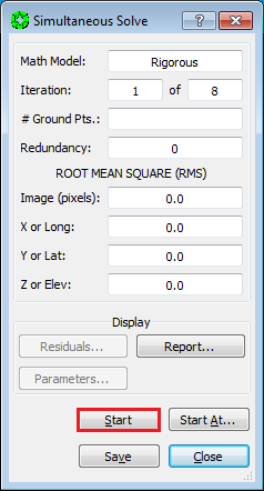
If the Image (pixels) RMS is < ~0.6 pixels, Press Save on the Simultaneous Solve window.
Press Yes on the Done pop-up window.
Press Close on the Simultaneous Solve window.
Select File > Exit on the Automatic Triangulation window.

Relative Orientation is now complete!

18.7. Re-Load Images

After the Relative Orientation is complete, it is necessary to re-Load the images in order to view them with the results of the adjustment. You should now have a parallax-free stereo model.

From the SOCET SET menu bar, select File > Load Images.
In the Image Loader window, select the Left and Right Image to display by clicking on the image id in the Left and Right panels. (Selected images will be highlighted.)
Under View Control Panel settings: Ensure that View = 1 and that Load Point is selected.
Press Load.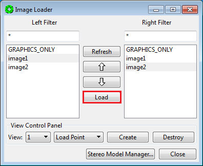
Press Close”

##18.8. Backup Relative Orientation Results

At this point, it is prudent for the operator to backup the project data in order to have a re-entry point that does not require the re-measure of tie points.

From the SOCET SET menu bar, select USGS Tools > Backup Orientation.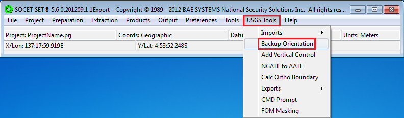
Make sure the current project name is listed in the Project field. If not, press “Project” to select the current project, then press “OK”. (Otherwise the backup will be made in, and for, the wrong project!)
Replace Backup_0 with _Relative in the Local folder name field. The backup folder will be named <ProjectName>_Relative.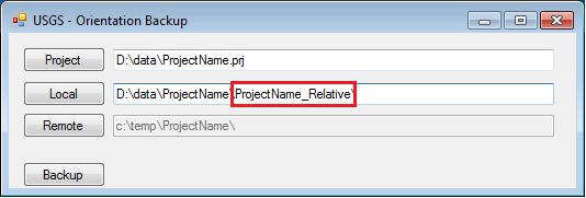
Press Backup.

19. Image Control Stage 2 - Vertical Adjustment to MOLA

19.1. Update Tie Points to Vertical (Z) Control

Utility “Add Vertical Control” adds elevation information based on MOLA heights to the tie points measured in the Relative Orientation. The tie points are then flagged as Z-Control points in the ground point file (GPF).

The “Add Vertical Control” utility will auto-fill the input files based on the <ProjectName> listed. If the grayed out entries are correct, simply check the boxes next to each field to confirm them. Otherwise, press the buttons associated with each field to select the correct files. The following steps detail the procedure.

From the SOCET SET menu bar, select USGS Tools > Add Vertical Control.
If the project file listed in the Project File field is correct, check the box next to the Project File field to confirm it. Otherwise, press the “Project File…” button to bring up the list of projects and select the project from the list.
The input ATF File should be <ProjectName>_Relative.atf. Either confirm the “ATF File” listed is correct by checking its check box, or press the “ATF File…” button to select <ProjectName>_Relative.atf. (The Ground Point File (GPF) is also listed. It should be <ProjectName>.gpf.)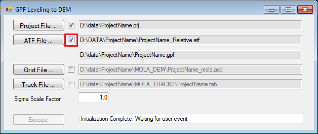
The input Grid File should be <ProjectName>_mola.asc located in the MOLA_DEM folder. Either confirm the Grid File listed is correct by checking its check box, or press the Grid File… button to select D:\\DATA\\<ProjectName>\\MOLA_DEM\\<ProjectName>_mola.asc.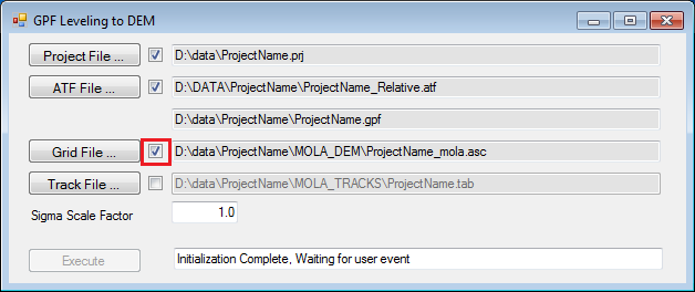
The input Track File should be <ProjectName>.tab located in the MOLA_TRACKS folder. Either confirm the Track File listed is correct by checking its check box, or press the Track File… button to select D:\\DATA\\<ProjectName>\\MOLA\_TRACKS\\<ProjectName>.tab. (Note: If a Track File does not exist, keep the Track File field blank and check the confirmation box.)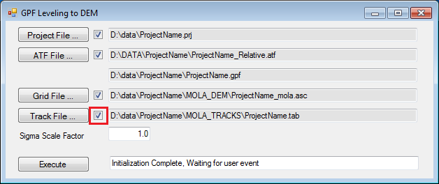
Press Execute. (If the Execute button is not activated please check the confirmation checkboxes.)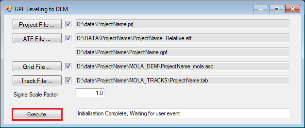
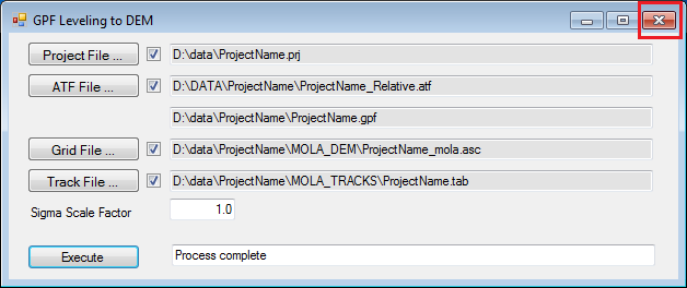
Close the window via the upper-right close button.

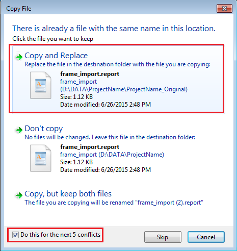
19.2. Restore Original (A-priori) Support Files

Open Windows Explorer. Navigate to D:\\DATA\\<ProjectName>\\<ProjectName>_Original, select all the files in the folder, and Copy them.

Note: There are more than image support files in this folder, but there is no harm copying the extraneous files, and it is quickest to just select all the files.
Move up one folder so you are now in D:\\DATA\\<ProjectName>, and paste the files.
In the pop-up window, check the box in the lower left corner to “do this for the next 3 conflicts”, then select “Copy and Replace”.
Close the Windows Explorer window.

19.3. Bundle Adjustment

From the SOCET SET menu bar, select Preparation > Multi-Sensor Triangulation.
Select File > Save Triangulation File As… in the Automated Triangulation window.

Note: <ProjectName>\_Relative.atf was automatically loaded. For the Vertical Adjustment to MOLA, no changes will be made to the Setup, however, we will provide a more meaningful name to the ATF file.
In the pop-up window, enter <ProjectName>_Rel_VertCtrl, and press OK.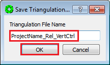
Press Solve in the Automated Triangulation window.
The Simultaneous Solve window will open, along with a Backup pop-up window. Press Yes on the pop-up to overwrite back up files.
In the Simultaneous Solve window, press Start to perform the bundle adjustment.
Once the adjustment is completed, evaluate the errors in the adjustment.

An acceptable solution has (1) an Image (pixels) RMS of ~0.6 or less, and (2)no individual point measurement has an error greater than 2 pixels.

Press Results button in the Simultaneous Solve window to review error of individual point measurements.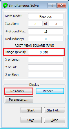
In the Vertical Adjustment procedure, all points are now Z-Control, so inspecting the top of the list will suffice.
If points have pixel errors greater than 2.0 pixels, SKIP TO: 18.4 Point Weights Refinement. Otherwise, continue to the next step.
If the image RMS is < ~0.6 pixels, and the maximum point measurement error is < 2.0 pixels, then Press Close on the Multi-Sensor Triangulation Residuals window.
Press Save on the simultaneous solve window.
Press Yes on the Done pop-up window.
Press Close on the Simultaneous Solve window.
Select File > Exit on the Automatic Triangulation window.

Vertical Adjustment is now complete!
SKIP: 18.4 Point Weight Refinement and 18.5 Point Re-Measurement Process, GO TO: 18.6 Re-Load Images.

19.4. Point Weights Refinement

Continuing from 18.3 Bundle Adjustment…

The previous Relative Orientation adjustment should have met the criteria of the Image RMS less than ~0.6 pixels, and individual point errors less than 2.0 pixels. The only change since the Relative Orientation is that we added elevation estimates to the measured points. If the Image RMS < ~0.6 pixels; Point Errors < 2.0 pixels criteria is not met now, the cause is most likely that the weights (i.e., Accuracy Values) assigned to the elevation estimates by “Add Vertical Control” are too stringent. We will first evaluate and adjust Accuracy values. If the criteria of an acceptable solution is still not met after another bundle adjustment (Solve), then we will re-measure points.

From the Multi-Sensor Triangulation Residuals window, record (on a piece of paper) the Point ID’s of the points with > 2.0 pixel line and/or sample errors. Then close the Residuals window.
Press Close on the Simultaneous Solve window. (Do not press Save.)
Press No to Saving Files in the Done pop-up window.
Press Interactive Point Measurement on the Automated Triangulation window.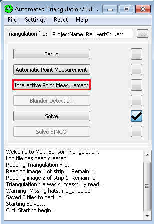
For each point recorded on your list:

a. Use the Scroll Bar to the right of the point list, and scroll to the point. Click on the point’s Point ID to select it.
```
![](media/image192.png)
```
b. IPM will move the stereo display to the selected point. Look at the measurement in stereo. If the point is on a slope, the Accuracy assigned to the Z coordinate may be too tight. We suggest you increase the Accuracy by approximately a factor of 2: double click in the Accuracy field for Z, delete the old value and type in the new value, then press the enter key.
When you are done updating Accuracy values, press Save then Close on the IPM window.
Press Solve on the Automated Triangulation window.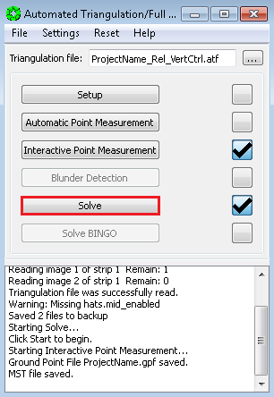
Press Start on the Simultaneous Solve window.
Press Residuals on the Simultaneous Solve window and make sure no individual point has an error greater than 2 pixels.
If the solution continues to have points with larger than 2 pixel errors, the problem may be a bad measurement(s), so GO TO 18.5 Point Re-Measurement Process. Otherwise, continue to the next step.
If the image RMS is < ~0.6 pixels, and the maximum point measurement error is < 2.0 pixels, we will exit Multi-Sensor Triangulation, and re-enter it in order to refresh the values stored in computer memory. First press Close on the Multi-Sensor Triangulation Residuals window.
Press Close on the Simultaneous Solve window (Do Not Press Save.)
Press No to Saving Files in the Done pop-up window.
Select File > Exit on the Automatic Triangulation window.
Re-enter MST: From the SOCET SET menu bar, select Preparation > Multi-Sensor Triangulation.
Press Solve on the Automatic Triangulation window. (The triangulation file, <ProjectName>_Rel_VertCtrl should load automatically.)
Press Yes on the pop-up to overwrite back up files.
Press Start on the Simultaneous Solve window.
If the Image (pixels) RMS is < ~0.6 pixels, Press Save on the Simultaneous Solve window.
Press Yes on the Done pop-up window.
Press Close on the Simultaneous Solve window.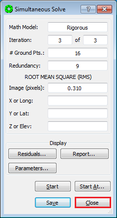
Select File > Exit on the Automatic Triangulation window.

Vertical Adjustment is now complete!
SKIP: 18.5 Point Re-Measurement Process, GO TO: 18.6 Re-Load Images.

19.5. Point Re-Measurement Process

Continuing from 18.4 Point Weights Refinement…

On the Multi-Sensor Triangulation Residuals window, Left-Click on the Point ID(s) of the points to re-measure. (Hold the Control Key down to select multiple points.) Then press Re-measure Point(s)…. The re-measure point window will now open with the points selected.
Left-Click on the point to re-measure. The View 1 (stereo display) window will display the current point measurement.
Un-check the Measured box for the Right image only, to remove parallax.

NOTE: Relocating the point is not advised because there is now an elevation estimate associated with the point.
Clear the parallax by moving the Right image only (i.e., put the dot on the ground).
Press Sample to collect the point measurement.
Press Save write the measurement to disk.
Repeat re-measurement process for remaining points in the list. (Go back to step 2.)
After points in the list are re-measured press Close.
Press Close on the Multi-Sensor Triangulation Residuals window.
Press Start on the Simultaneous Solve window.
Press Residuals on the Simultaneous Solve window and make sure no individual point has an error greater than 2 pixels.
If there are points with larger than 2 pixel errors, repeat the Point Re-Measurement Process starting from step 1.
If the image RMS is < ~0.6 pixels, and the maximum point measurement error is < 2.0 pixels, we will exit Multi-Sensor Triangulation, and re-enter it in order to refresh the values stored in computer memory. First press Close on the Multi-Sensor Triangulation Residuals window.
Press Close on the Simultaneous Solve window (Do Not Press Save.)
Press No to Saving Files in the Done pop-up window.
Select File > Exit on the Automatic Triangulation window.
Re-enter MST: From the SOCET SET menu bar, select Preparation > Multi-Sensor Triangulation.
Press Solve on the Automatic Triangulation window. (The triangulation file, <ProjectName>_Rel_VertCtrl should load automatically.)
Press Yes on the pop-up to overwrite back up files.
Press Start on the Simultaneous Solve window.
If the Image (pixels) RMS is < ~0.6 pixels, Press Save on the Simultaneous Solve window.
Press Yes on the Done pop-up window.
Press Close on the Simultaneous Solve window.
Select File > Exit on the Automatic Triangulation window.

.

Vertical Adjustment to MOLA is now complete!

19.6. Re-Load Images

After the Vertical Adjustment to MOLA is complete, it is necessary to re-Load the images in order to view them with the results of the adjustment.

From the SOCET SET menu bar, select File > Load Images`.
In the Image Loader window, select the Left and Right Image to display by clicking on the image id in the Left and Right panels. (Selected images will be highlighted.)
Under View Control Panel settings: Ensure that View = 1 and that Load Point is selected.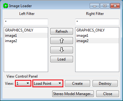
Press Load.

![](media/image234.png)

Press Close.

19.7. Backup Vertical Adjustment Results

At this point, it is prudent to backup the project data in order to have a re-entry point for the up-coming Absolute Orientation of the stereo images to MOLA.

From the SOCET SET menu bar, select USGS Tools > Backup Orientation.
Make sure the current project name is listed in the Project field. If not, press “Project” to select the current project, then press OK. (Otherwise the backup will be made in, and for, the wrong project!)
Replace Backup_0 with Relative_VerticalControl in the Local folder name field. The backup folder will be named <ProjectName>_Relative_VerticalControl.
Press Backup.

20. Image Control Stage 3 - Absolute Orientation

20.1. Overview

The objective of this stage is to better align the stereo model to the surface topography represented by the MOLA tracks. This step is highly subjective in nature and the analyst should look for “trends” in the stereo model not fitting the altimetry tracks. The goal will be to look for shifts in the XY plane and to identify the movement required to make the entirety of the stereo coverage align the tracks properly through the use of horizontal control gathered from the MOLA Tracks.

Subjectively picking horizontal control is not an exact process, so we will use a single horizontal control point to translate the stereo pair in alignment with the MOLA Tracks. Using more than one horizontal control point can distort (buckle, twist, stretch) the stereo model if multiple points are inaccurate.

If there are not adequate MOLA Track data for horizontal control (either the MOLA tracks are too sparse, or the terrain is too flat to tie a feature to an XY location) we will stop the controlling process and use the “dead-reckoning” results of the Vertical Alignment. (Note that in the Vertical Alignment, horizontal positioning is controlled by holding the nadir-most image, and accurate to the level of the nadir-most image’s position and pointing accuracy.)

NOTE:

In this procedure, we will use the Feature Extraction, Coordinate Measurement and Multi-Sensor Triangulation tools. Many windows will be open, so try to arrange them on the console monitor to allow easy access between tools.
You may also encounter erroneous MOLA Tracks that appear out of alignment with surrounding tracks. The erroneous tracks should be ignored.

20.2. Evaluate MOLA Tracks for Horizontal (XYZ) Control

From the SOCET SET menu bar, select Extraction > Feature > Feature Extraction.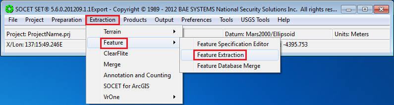
From the Feature Extraction window select File > Open FDB….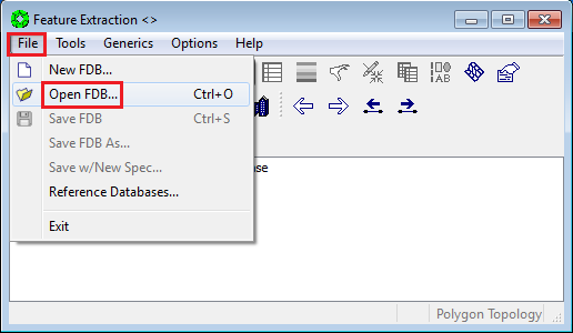
Select <ProjectName>_mola_tracks, and press OK.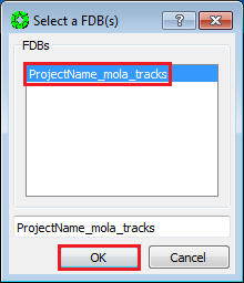
Make sure Auto-Draw is on. Press the Auto-Draw icon until it appears in a depressed state.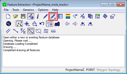
Using the Zoom In or Zoom out buttons on the TopoMouse, set the Zoom Level to 16:1 in order to have an overview of the relief of the tracks and the relief in the stereo model.
Roam the stereo model to discern if horizontal movement of the stereo images would better align the stereo model to the altimetry (e.g., MOLA) tracks.

Note: The images loaded must be from the Vertical Alignment solution so that the tracks are closer to the stereo surface vertically.
If no trend in terrain shift can be identified, then the Image Control process is complete. Close the Feature Extraction window, and SKIP to 20 Epipolar (Pair-Wise) Rectify Controlled Images.

20.3. Determine Horizontal Control Point

Continue on in Feature Extraction to identify a horizontal control point as follows:

Roam the stereo model and visually correlate a distinguishable trend in one of the MOLA tracks (e.g., the tracks going over a ridge), with a distinguishable feature in the stereo model (e.g., a ridge). Zoom-In and Zoom-Out during the search for these features.
In the identified trend, choose a single MOLA track point to tie to a distinguishable correlated feature in the stereo model.
From the SOCET SET menu bar, select Tools > Coordinate Measurement. (We will use Coordinate Measurement to store the coordinates of the MOLA Track point to be used for XYZ control.)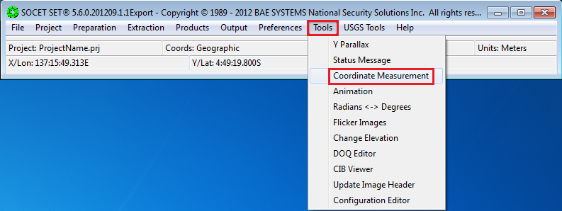
On the View1 (stereo display window), press the Refresh Graphics icon to remove the anchor point drawn by Coordinate Measurement. Wait for the MOLA Tracks to re-draw.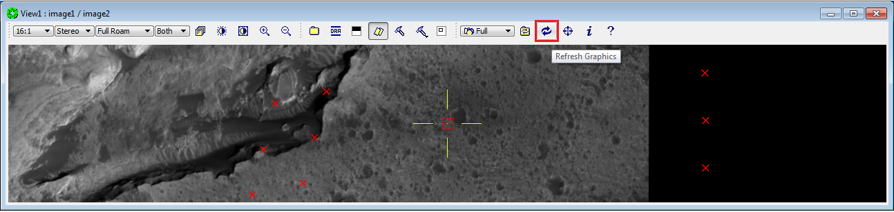
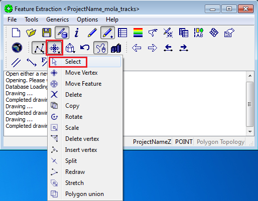
In the Feature Extraction window, hold the Edit icon down to display a menu of available Edit Tools. Select the Select tool.

Note: The Edit icon will now appear as a white arrow and should be seen in a depressed state. The extraction cursor on the stereo display has also changed in color to white.
Move the extraction cursor close to the MOLA Track point of interest (i.e., the one that is correlated with a feature in the stereo model.) Zoom to 1:1 and refine the placement of the extraction cursor if needed.
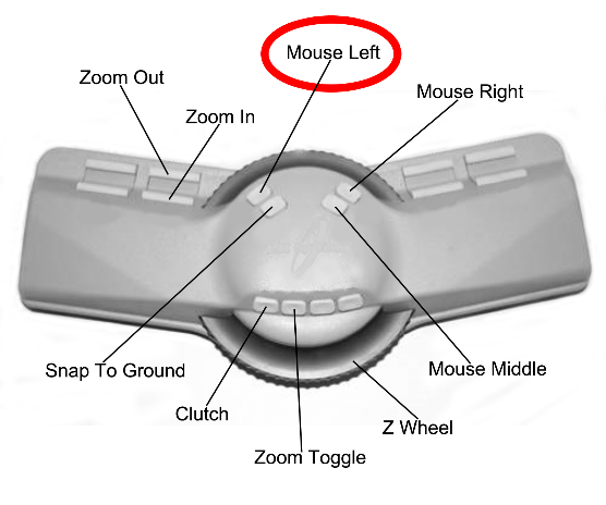
Press the Left Mouse button on the TopoMouse to select the track point.

The extraction cursor will jump to the MOLA Track point, and the selected track point will be displayed as white.
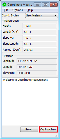
DO NOT MOVE THE TOPOMOUSE. (If you think you moved it, re-select the track point before proceeding.) On the Coordinate Measurement window, select Capture Point. This will record the longitude, latitude and elevation of the selected MOLA track point in the report section of the Coordinate Measurement window.
On the Coordinate Measurement Tool window, select “Options” > “Move To Point”.

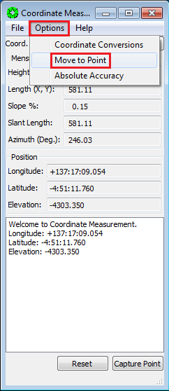
The Move To Point window will appear, populated with the coordinates of the MOLA Track point.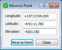

20.4. Absolute Orientation Setup

From the SOCET SET menu bar, select Preparation > Multi-Sensor Triangulation.
Select File > Save Triangulation File As… in the Automated Triangulation window.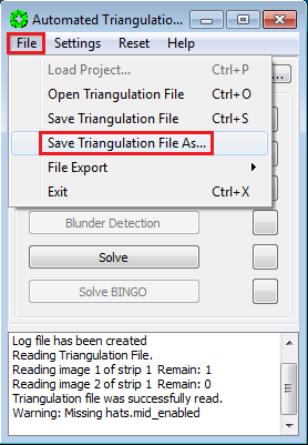
In the pop-up window, enter <ProjectName>_Abs_XYZ_Ctrl, and press OK.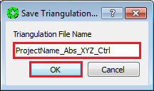
Press Setup on the Automated Triangulation window. We will be setting up image parameters for an Absolute Orientation (where both images will be allowed to adjust.)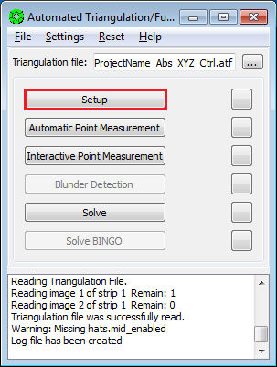
In the Setup window, select the oblique image of the stereo pair, and press Image Data….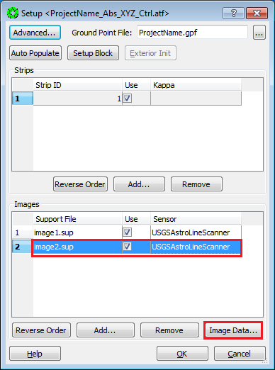
Insure the Adjustable Image Parameters are as shown, Press the radio button for All Images, and then press OK. (These adjustable parameters will be copied to the nadir-most image.)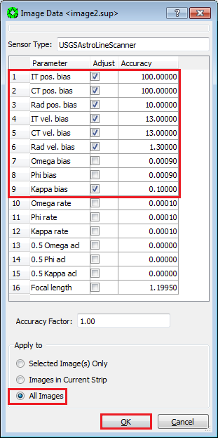

Parameter Accuracy

IT pos. bias 100 m

CT pos. bias 100 m

Radial pos. bias 10 m

IT vel. bias 13 m/s

CT vel. bias 13 m/s

Radial vel. bias 1.3 m/s

Kappa bias 0.1 degree

20.5. Measure Horizontal Control Point

Press Interactive Point Measurement on the Automated Triangulation window.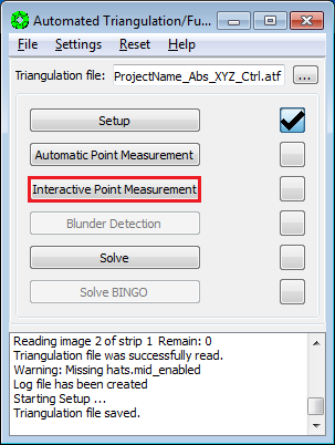
Press Settings in the Interactive Point Measurement (IPM) window.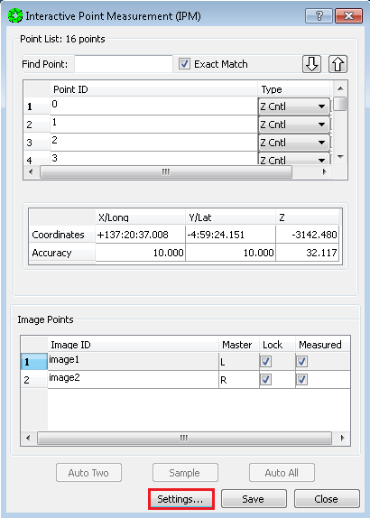
In the Settings for IPM window, make sure the Auto Img List box is checked, then press Close.
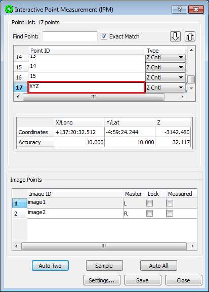
Right Click in the Point ID field, and Select Add in the pop-up window.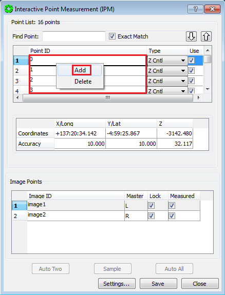
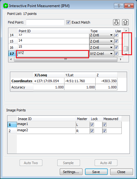
IPM will automatically scroll to the bottom of the list to where the new point is added. Double left-click on the Point ID of the new point to enable editing the default id. Replace the current id (e.g., 16) with XYZ and press the enter key.
For this new point, click on its Type field (i.e., the box that says Z Ctrl) to bring up the Point Type Options. Select XYZ Ctrl from the list of options.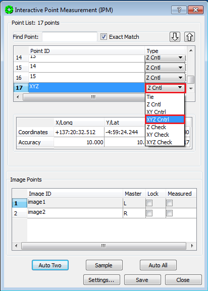
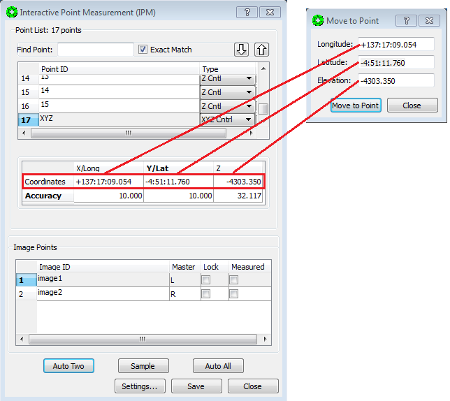
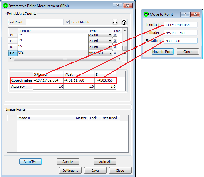
From the Move To Point window, Copy the Longitude, Latitude and Elevation coordinates, and Paste them into the Coordinates fields for the XYZ point. Make sure not to leave behind any negative signs. (Alternatively, you can copy the captured coordinates listed in the Coordinate Measurement window.)
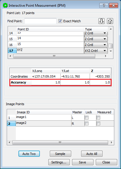
Set the Accuracy values for the Longitude, Latitude and Z coordinates to 1 meter each. (We are going to hold to this coordinate tightly.)
On the Move To Point window, press Move To Point. This will move the extraction cursor to the location of the selected MOLA Track point. (The selected track point will still be colored white.)
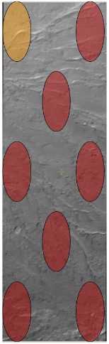
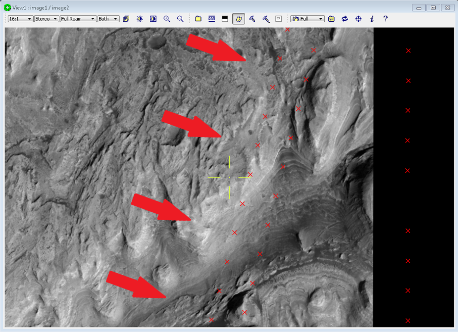
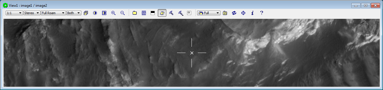
Place the extraction cursor on the feature in the stereo model you want to correlate with the selected track point. (Make sure the extraction cursor is on the ground.)

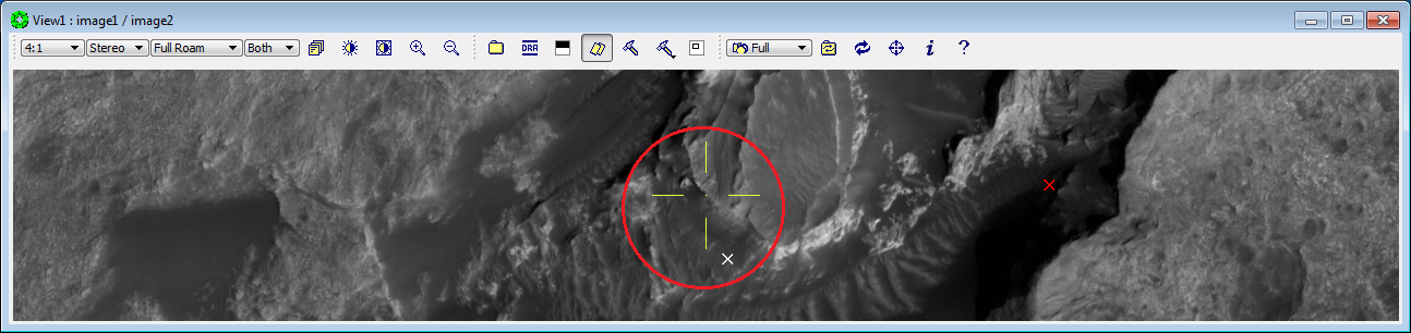
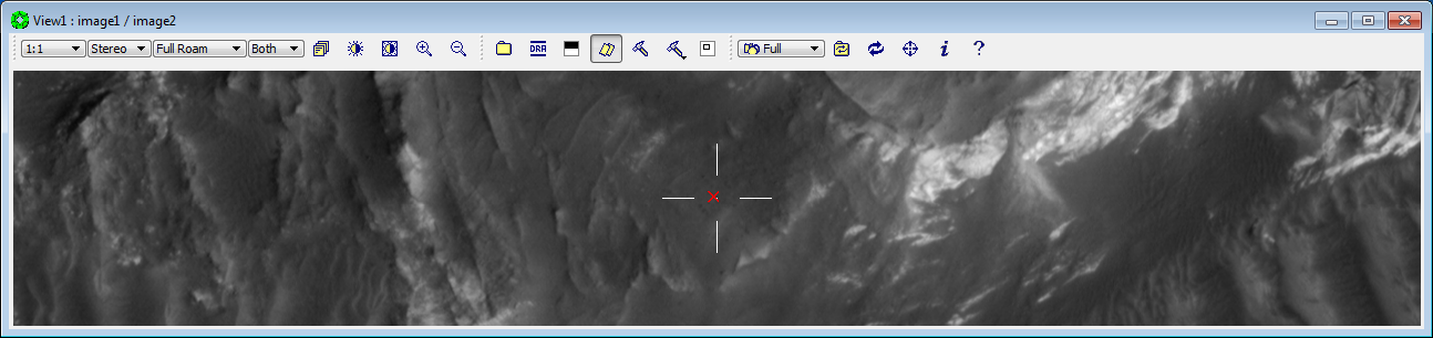
In the following figure, the area circled in red shows an example of a selected track point (the white x), and the location of a feature to correlate with the track point (the center of the yellow extraction cursor).
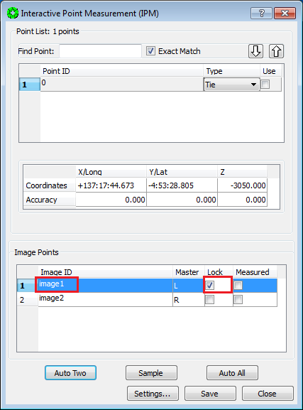
In the IPM window, lock the Left image by checking the Lock box.
Refine the parallax removal (at ground level) by moving the Right image only. In other words, put the dot on the ground.
Press Sample on the IPM window to collect the point measurement.
Press Save on the IPM window to write the measurement to disk. Then press Close.
Select File > Exit on the Automated Triangulation window.

20.6. Iterative Steps to Fine-Tune XYZ Control Point

The following steps, preceded with **, are iterative. The process stops when you have established an XYZ Control point that aligns the stereo model to the MOLA tracks at a level that meets your needs.

20.6.1. **Restore Original (A-Priori) Support Files

Open Windows Explorer. Navigate to D:\\DATA\\<ProjectName>\\<ProjectName_Original, select all the files in the folder, and Copy them.
Move up one folder so you are now in D:\\DATA\\<ProjectName>, and paste the files.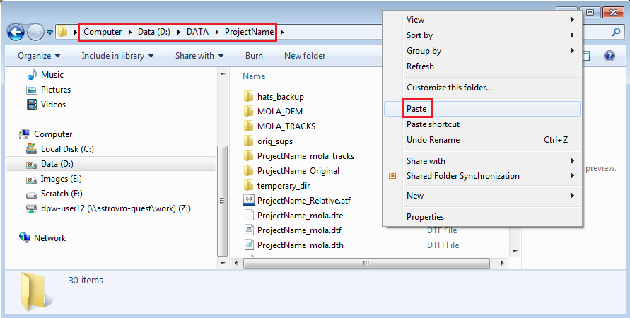
In the pop-up window, check the box in the lower left corner to “do this for the next 3 conflicts”, then select Copy and Replace.
Close the Windows Explorer window.

20.6.2. **Bundle Adjust

From the SOCET SET menu bar, select Preparation > Multi-Sensor Triangulation
In the Automated Triangulation window, press Solve. (Note that <ProjectName>_Abs_XYZ_Ctrl was automatically loaded.)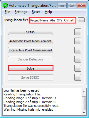
Press Yes on the pop-up to overwrite back up files.
Press Start in the Simultaneous Solve window.
If the Image Pixels RMS has not blown up (e.g., it is under 1 pixel), press Save on the simultaneous solve window.

Note: Because finding the image location of the XYZ (track) point is iterative, getting a “perfect” solution at each iteration is not efficient. Later on we will evaluate the individual point errors.

If the Image RMS is more than 1 pixel, the likely problem is that the XYZ Control point is mis-measured or has an error in its Coordinates. To check it, press “Close” on the “Simultaneous Solve” window; select “No” for saving files, then go back into IPM to check the XYZ point.
Press Yes on the Done pop-up window.
Press Close on the Simultaneous Solve window.

20.6.3. **Re-Load Images

It is necessary to Re-Load the images in order to view the stereo images with the results of the horizontal adjustment.

From the SOCET SET menu bar, select File > Load Images.
In the Image Loader window, select the Left and Right Image to display by clicking on the image id in the Left and Right panels. (Selected images will be highlighted.)
Under View Control Panel settings: Ensure that View = 1 and that Load Point is selected.
Press Load.
Press Close.

![](media/image289.png)

20.6.4. **Evaluate Horizontal Shift of Stereo Model

Roam the stereo model to evaluate the new alignment of the stereo model to the MOLA Tracks. Now that the stereo model is closer to truth, it should be easier to decide how to further move the stereo model to better align it with the MOLA Tracks. You will have three options:

a. If you want to tweak the placement (image measurement) of the currently selected track point: GO TO 19.6.5 Re-Position Current Horizontal Control Point.

b. If you want to select a different track point for horizontal control: GO TO 19.6.6 Select Different Horizontal Control Point

c. If the alignment is satisfactory:
1. Press Close on the Move to Point window.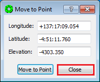
2. Select File > Exit on the Coordinate Measurement window.
```
![](media/image291.png)
```
1. Select File > Exit on the Feature Extraction window.
```
![](media/image292.png)
```
1. GO TO 19.7 Update Vertical (Z) Control.

20.6.5. **Re-Position Current Horizontal Control Point

Press Interactive Point Measurement on the Automated Triangulation window.
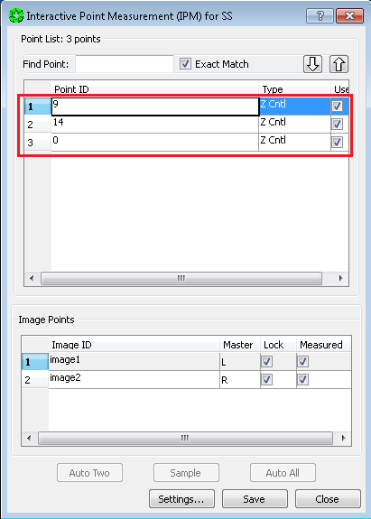
Use the Scroll Bar to the right of the point list, and scroll to the bottom of the list. Click on the Point ID of the XYZ Control point to select it. (IPM will move the stereo display to the measured point.)
Un-check the boxes in the Measured field for both images. (This will also unlock both images so that point can be measure at another location.)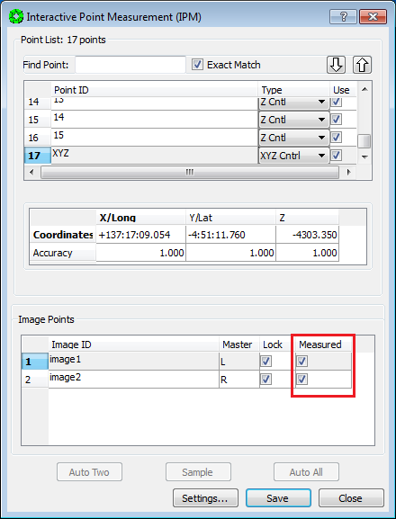
Place the extraction cursor on the new location/feature in the stereo model you want to correlate with the selected track point. (Make sure the extraction cursor is also on the ground.)
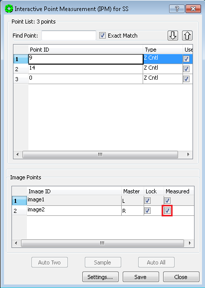
In the IPM window, lock the Left image by checking its Lock box.
Refine the parallax removal (at ground level) by moving Right image only. In other words, put the dot on the ground.
Press Sample on the IPM window to collect the point measurement.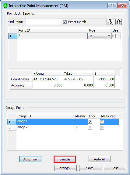
Press Save on the IPM window to write the measurement to disk. Then press Close.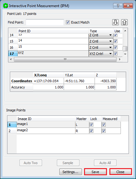
Select File > Exit on the Automated Triangulation window.
GO TO 19.6.1 **Restore Original (A-Priori) Support Files, and reiterate.

20.6.6. **Select Different Horizontal Control Point

Close the Move To Point window (but keep the Coordinate Measurement tool running.)
Roam the stereo model and visually correlate a distinguishable trend in one of the MOLA tracks (e.g., the tracks going over mound), with a distinguishable feature in the stereo model (e.g., a mound). Zoom-In and Zoom-Out during the search for these features.
In the identified trend, choose a single MOLA track point to “tie” to a distinguishable correlated feature in the stereo model.
Press the On-Line icon on the Feature Extraction window. This will give control of the extraction cursor back to the Feature Extraction Tool.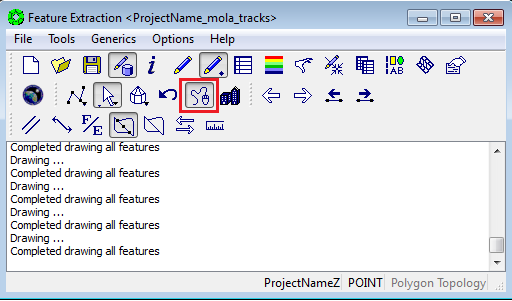

Note: Interactive Point Measurement (IPM) takes automatic control of the extraction cursor and IPM cannot be running when we use the Feature Extraction tool. If IPM is running, you must exit it before returning to the Feature Extraction tool. There is no conflict if the main Automated Triangulation window remains open.
Move the extraction cursor close to the MOLA Track point of interest (i.e., one that is correlated with a feature in the stereo model.) Zoom to 1:1 and refine the placement of the extraction cursor if needed.
Press the Left Mouse button on the TopoMouse to select the track point.

The extraction cursor will jump to the MOLA Track point, and the selected track point will be displayed as white.
DO NOT MOVE THE TOPOMOUSE. (If you think you moved it, re-select the track point before proceeding.) On the Coordinate Measurement window, select Capture Point. This will record the longitude, latitude and elevation of the selected MOLA track point in the report section of the Coordinate Measurement window.
On the Coordinate Measurement Tool window, select Options > Move To Point.

The Move To Point window will appear, populated with the coordinates of the MOLA Track point.
Press Interactive Point Measurement on the Automated Triangulation window.
Use the Scroll Bar to the right of the point list, and scroll to the bottom of the list. Click on the Point ID of the XYZ Control point to select it. (IPM will move the stereo display to the measured point.)
From the Move To Point window, copy the Longitude, Latitude and Elevation coordinates, and Paste them into the Coordinates fields for the XYZ point. Make sure not to leave behind any negative signs. (Alternatively, you can copy the captured coordinates listed in the Coordinate Measurement window.)
Un-check the boxes in the Measured field for both images. (This will also unlock both images so that point can be measure at another location.)
On the Move To Point window, press Move To Point. This will move the extraction cursor to the location of the selected MOLA Track point. (The selected track point will still be colored white.)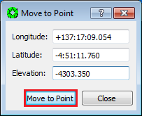
Place the extraction cursor on the feature in the stereo model you want to correlate with the selected track point. (Make sure the extraction cursor is also on the ground.)
In the IPM window, lock the Left image by checking its Lock box.
Refine the parallax removal (at ground level) by moving Right image only. In other words, put the dot on the ground.
Press Sample on the IPM window to collect the point measurement.
Press Save on the IPM window to write the measurement to disk. Then press “Close”.
Select File > Exit on the Automated Triangulation window.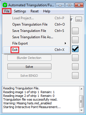
GO TO 19.6.1 **Restore Original (A-Priori) Support Files, and reiterate.

20.7. Update Vertical (Z) Control

Because we have shifted the stereo model horizontally, we must correct the elevation estimates of the Z Control points.

From the SOCET SET menu bar, select USGS Tools > Add Vertical Control.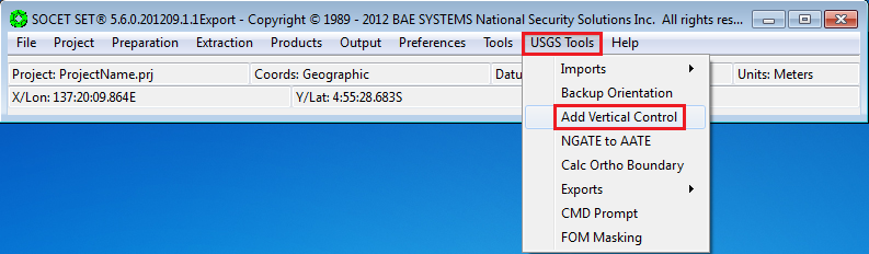
If the project file listed in the Project File field is correct, check the box next to the Project File field to confirm it. Otherwise, press the Project File… button to bring up the list of project files, and select <ProjectName>.prj from the list.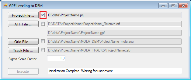
Press ATF File…. (We must select the current ATF file.)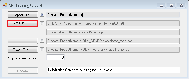
In the Open window, select <ProjectName>_Abs_XYZ_Ctrl, and then press Open.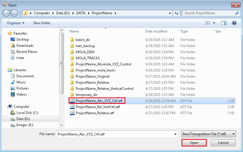
The input Grid File should be <ProjectName>_mola.asc located in the MOLA_DEM folder. Either confirm the “Grid File” listed is correct by checking its check box, or press the Grid File… button to select D:\\DATA\\<ProjectName>\\MOLA_DEM\\<ProjectName>_mola.asc.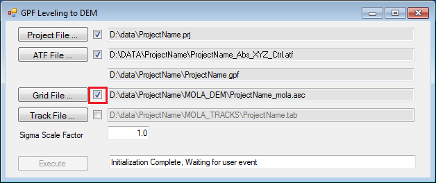
The input Track File should be <ProjectName>.tab located in the MOLA_TRACKS folder. Either confirm the Track File listed is correct by checking its check box, or press the Track File… button to select D:\\DATA\\<ProjectName>\\MOLA_TRACKS\\<ProjectName>.tab.
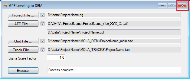
Press Execute. (If the Execute button is not activated please check the confirmation checkboxes.)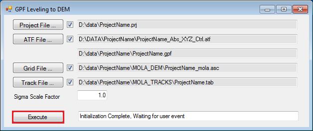
Close the GUI via the close icon.

20.8. Restore Original (A-priori) Support Files

Open Windows Explorer. Navigate to D:\\DATA\\<ProjectName>\\<ProjectName_Original, select all the files in the folder, and Copy them.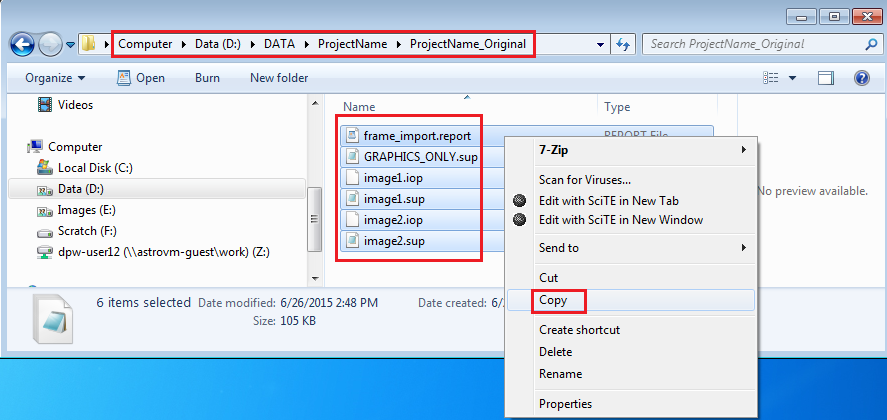
Move up one folder so you are now in D:\\DATA\\<ProjectName>, and paste the files.
In the pop-up window, check the box in the lower left corner to “do this for the next 3 conflicts”, then select Copy and Replace.
Close the Windows Explorer window.

20.9. Final Bundle Adjustment

From the SOCET SET menu bar, select Preparation > Multi-Sensor Triangulation.
In the Automated Triangulation window, press Solve.
Press Yes on the pop-up to overwrite back up files.
Press Start in the Simultaneous Solve window.
Once the adjustment is completed, evaluate the errors in the adjustment.

An acceptable solution has (1) an Image (pixels) RMS of ~0.6 or less, and (2) no individual point measurement has an error greater than 2 pixels.

Press Results button in the Simultaneous Solve window to review error of individual point measurements
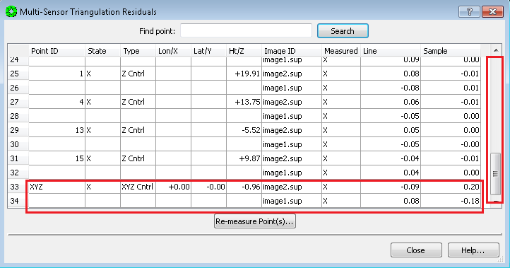
Points in the Residuals window are grouped by Type, and automatically sorted from highest to lowest residual within each Type category. The Line and Sample fields list the point measurement errors in pixels. In the Absolute Orientation procedure, there is a mix of Z-Control and XYZ-Control points, so scroll through the list to each section looking for unacceptable point measurement errors.
If points have pixel errors greater than 2.0 pixels, GO TO: 19.10 Point Weights Refinement. Otherwise, continue to next step.
If the image RMS is < ~0.6 pixels, and the maximum point measurement error is < 2.0 pixels, then Press Close on the Multi-Sensor Triangulation Residuals window.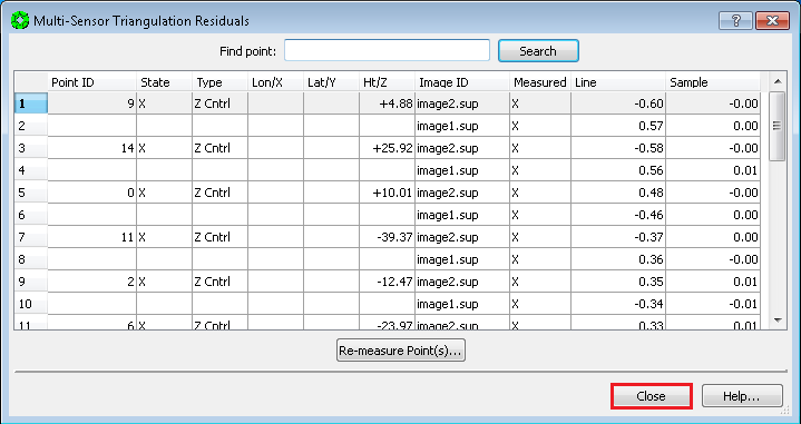
Press Save on the Simultaneous Solve window.
Press Yes on the Done pop-up window.
Press Close on the Simultaneous Solve window.
Select File > Exit on the Automatic Triangulation window.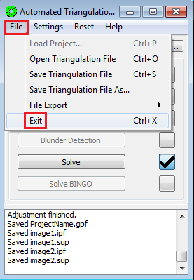

Absolute Orientation is now complete!
SKIP: 19.10 Point Weights Refinement and 19.11 Point Re-Measurement Process, GO TO: 19.12 Re-Load Images.

20.10. Point Weights Refinement

Continuing from 19.9 Final Bundle Adjustment…

We have now updated the elevation estimates to the Z-Control points. If the Image RMS < ~0.6 pixels; and Point Errors < 2.0 pixels criteria has not been met, the cause may be that the weights (i.e., Accuracy Values) assigned to the elevation estimates by “Add Vertical Control” are too stringent. We will first evaluate and adjust Accuracy values. If the criteria of an acceptable solution is still not met after another bundle adjustment (Solve), then we will re-measure points.

From the Multi-Sensor Triangulation Residuals window, record (on a piece of paper) the Point ID’s of the points with > 2.0 line/sample errors. Then close the Residuals window.
Press Close on the Simultaneous Solve window. (Do not press Save.)
Press No to Saving Files in the Done pop-up window.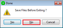
Press Interactive Point Measurement on the Automated Triangulation window.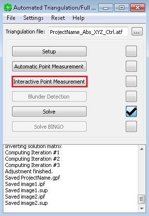
For each point recorded on your list:

a. Use the Scroll Bar to the right of the point list, and scroll to the point. Click on the point’s Point ID to select it.

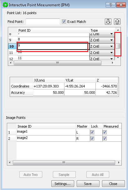
b. IPM will move the stereo display to the point. Look at the measurement in stereo. If the point is on a slope, the Weight/Accuracy assigned to the Z coordinate may be too tight. We suggest you increase the accuracy by approximately a factor of 2: double click in the Accuracy field for Z, delete the old value and type in the new value, then press the enter key.
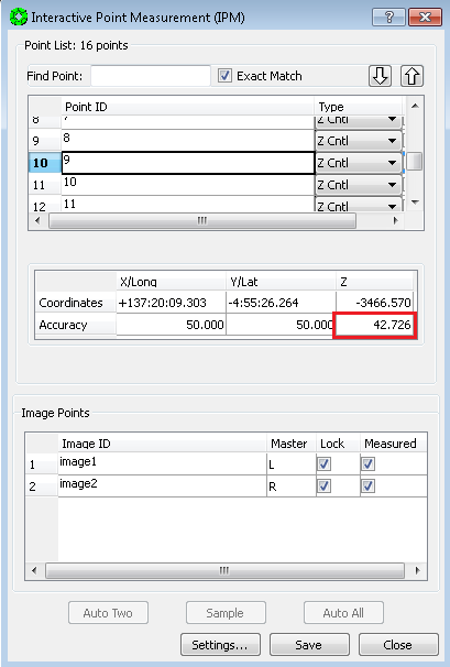
When you are done updating Accuracy values, press Save then Close on the IPM window.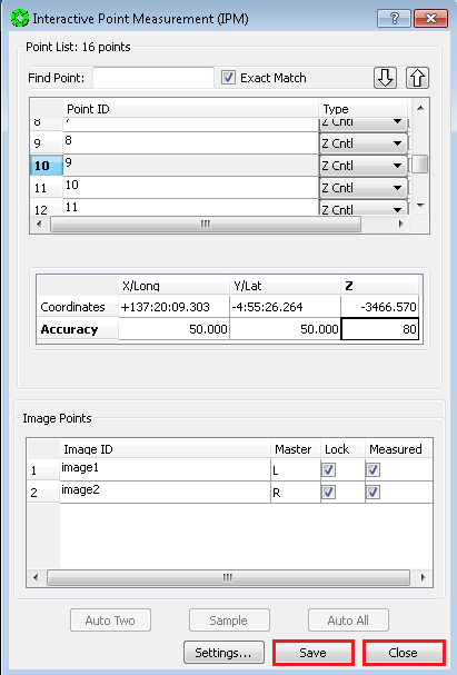
Press Solve on the Automated Triangulation window.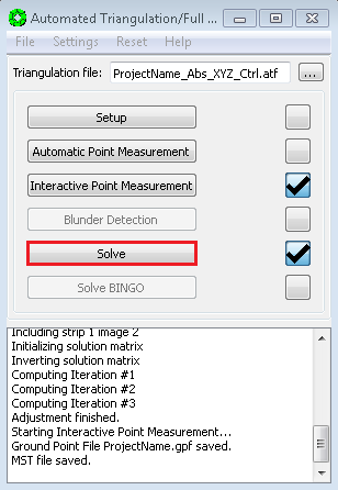
Press Start on the Simultaneous Solve window.
Press Residuals on the Simultaneous Solve window and make sure no individual point has an error greater than 2 pixels.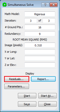
If the solution continues to have points with larger than 2 pixel errors, the problem may be a bad measurement(s), so GO TO 19.11 Point Re-Measurement Process. Otherwise, continue to next step.
If the image RMS is < ~0.6 pixels, and the maximum point measurement error is < 2.0 pixels, we will exit Multi-Sensor Triangulation, and re-enter it in order to refresh the values stored in computer memory. First press Close on the Multi-Sensor Triangulation Residuals window.
Press Close on the Simultaneous Solve window. (Do Not Press Save.)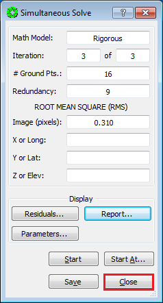
Press No to Saving Files in the Done pop-up window.
Select File > Exit on the Automatic Triangulation window.
Re-enter MST: From the SOCET SET menu bar, select Preparation > Multi-Sensor Triangulation.
Press Solve on the Automatic Triangulation window.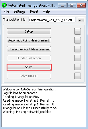
Press Yes on the pop-up to overwrite back up files.
Press Start on the Simultaneous Solve window.
If the Image (pixels) RMS is < ~0.6 pixels, Press Save on the Simultaneous Solve window.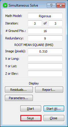
Press Yes on the Done pop-up window.
Press Close on the Simultaneous Solve window.
Select File > Exit on the Automatic Triangulation window.

Absolute Orientation is now complete!
SKIP: 19.11 Point Re-Measurement Process, GO TO: 19.12 Re-Load Images.

20.11. Point Re-Measurement Process

Continuing from 19.10 Point Weights Refinement…

On the Multi-Sensor Triangulation Residuals window, Left-Click on the Point ID(s) of the points to re-measure. (Hold the Control Key down to select multiple points.) Then press Re-measure Point(s)…. The re-measure point window will now open with the points selected.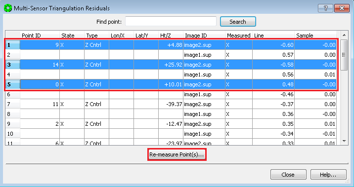
Left-Click on the point to re-measure. The View 1 (stereo display) window will display the current point measurement.
Un-check the Measured box for the Right image only, to remove parallax.

NOTE: Relocating the point is not advised because an elevation estimate is associated with the point.
Clear the parallax by moving the Right image only (i.e., put the dot on the ground).
Press Sample to collect the point measurement.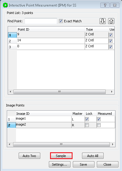
Press Save to write the measurement to disk.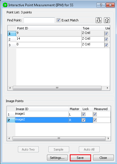
Repeat re-measurement process for remaining points in the list. (Go back to step 2.)
Press Close after all points in the list are re-measured.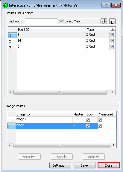
Press Close on the Multi-Sensor Triangulation Residuals window.
Press Start on the Simultaneous Solve window.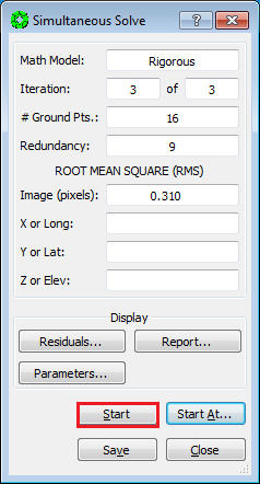
Press Residuals on the Simultaneous Solve window and make sure no individual point has an error greater than 2 pixels.
If there are points with larger than 2 pixel errors, repeat the 19.11 Point Re-Measurement Process from step 1.
If the image RMS is < ~0.6 pixels, and the maximum point measurement error is < 2.0 pixels, we will exit Multi-Sensor Triangulation, and re-enter it in order to refresh the values stored in computer memory. First press Close on the Multi-Sensor Triangulation Residuals window.
Press Close on the Simultaneous Solve window. (Do not press Save.)
Press No to Saving Files in the Done pop-up window.
Select File > Exit on the Automatic Triangulation window.
Re-enter MST: From the SOCET SET menu bar, select Preparation > Multi-Sensor Triangulation.
Press Solve on the Automatic Triangulation window.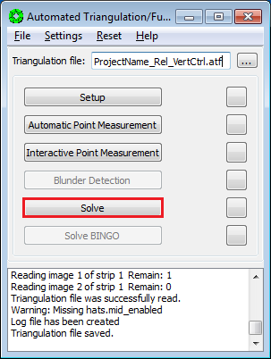
Press Yes on the pop-up to overwrite back up files.
Press Start on the Simultaneous Solve window.
If the Image (pixels) RMS is < ~0.6 pixels, Press Save on the Simultaneous Solve window.
Press Yes on the Done pop-up window.
Press Close on the Simultaneous Solve window.
Select File > Exit on the Automatic Triangulation window.

Absolute Orientation is now complete!

20.12. Re-Load Images

After the Absolute Orientation is complete, it is necessary to re-Load the images in order to view them with the results of the adjustment.

From the SOCET SET menu bar, select File > Load Images.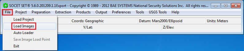
In the Image Loader window, select the Left and Right Image to display by clicking on the image id in the Left and Right panels. (Selected images will be highlighted.)
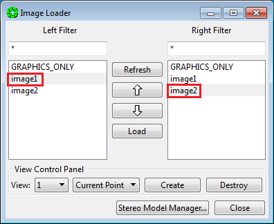
Under View Control Panel settings: Ensure that View = 1 and that Load Point is selected.
Press Load.
Press Close.

20.13. Backup Absolute Orientation Results

From the SOCET SET menu bar, select USGS Tools > Backup Orientation.
Make sure the current project name is listed in the Project field. If not, press “Project” to select the current project, then press “OK”. (Otherwise the backup will be made in, and for, the wrong project!)
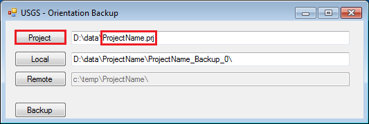
Replace Backup_0 with Absolute_XYZ_Control in the Local folder name field. The backup folder will be named <ProjectName>_Absolute_XYZ_Control.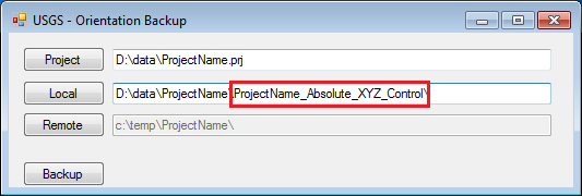
Press Backup.

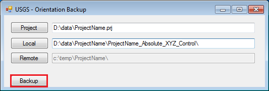
21. Epipolar (Pair-Wise) Rectify Controlled Images

Epipolar rectification is used to enhance or enable stereo visualization of a stereo image pair. This rectification process: rotates the images so the epipolar (e.g., X-parallax) direction is horizontal, and scales the images to a common resolution.

Generally, SOCET SET can handle epipolar rectification on-the-fly (also referred to as Pairwise Rectification in the SOCET SET user’s manual). Although on-the-fly rectification works for viewing pushbroom/linescanner stereo images, it is unreliable when automatically generating a DTM. Therefore, we need to generate epipolar (pair-wise) rectified images of the stereo pair and supply them to NGATE (Next Generation Automatic Terrain Extraction) and AATE (Adaptive Automatic Terrain Extraction).

##21.1. Load Controlled Images

Load the images to insure the stereo display is using the final controlled solution of the images.

From the SOCET SET menu bar, select File > Load Images
In the Image Loader window, select the Left and Right Image to display by clicking on the image id in the Left and Right panels. (Selected images will be highlighted.)
Under View Control Panel settings: Ensure that View = 1 and that Load Point is selected.
Press Load.
Press Close.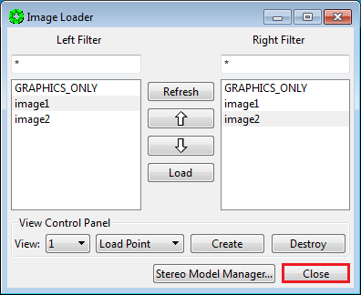

21.2. Generate Epipolar Rectified Images

From the SOCET SET menu bar, select Preparation > Resample > Rectification > Pair-Wise.

![](media/image397.png)

In the Pairwise Rectification window, verify the Output Image section is correct. Then press Start.

SOCET SET will automatically populate this GUI based on the stereo pair loaded. Just make sure the Output Image Location is correct. The output image names are based are the left and Right images loaded, and will have _l and _r appended.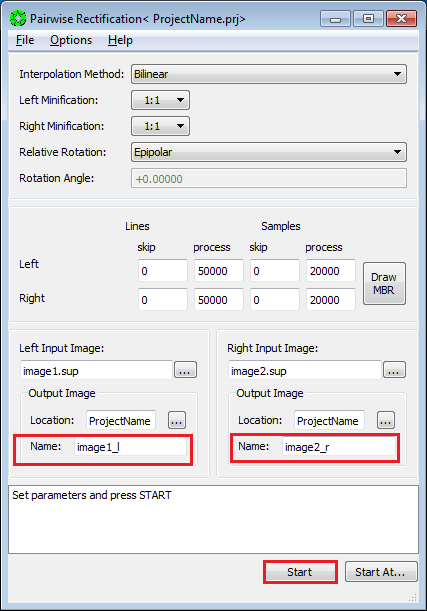
Upon completion, Select File > Exit in the Pairwise Rectification window

22. Generate DTM

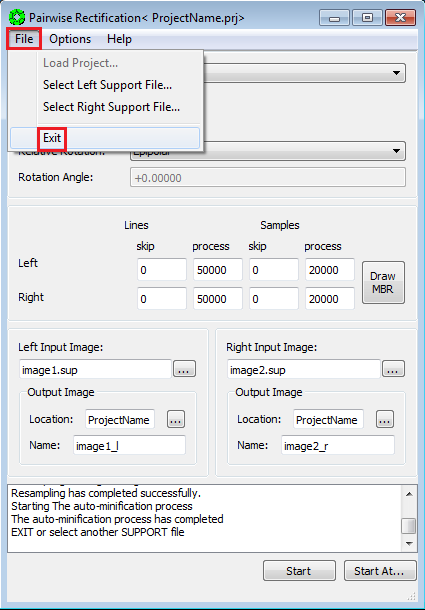
For HiRISE, both NGATE and AATE are used to generate a one meter post DTM. In stereo pairs with substantial relief, and when the stereo images are controlled to the MOLA (either from the Vertical Adjustment or the Absolute Orientation), we use the MOLA DTM as a seed file. This closer approximation to ground-truth greatly increases success of the matcher. In stereo pairs of flat terrain, seeding with MOLA is not necessary.

22.1. Load Epipolar Rectified Images

From the SOCET SET menu bar, select File > Load Images.
In the Image Loader window, select <image1>_l for the Left image, and <image1>_r for the Right Image.
Under View Control Panel settings: Ensure that View = 1 and that Load Point is selected.
Press Load.
Press Close.

22.2. Next Generation Automatic Extraction (NGATE)

From the SOCET SET menu bar, select Extraction > Terrain > Next Generation Automatic Extraction.

22.2.1. Create a New DTM

In the NGATE window, select File > Create DTM. (This will bring up the Create DTM window.)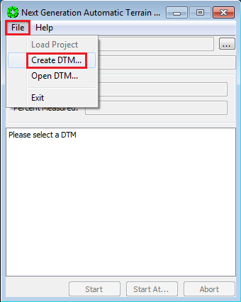
In the Create DTM window, press the box next to the DTM field.
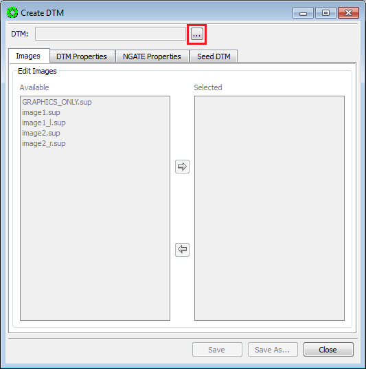
In the Select a DTM window, hand enter the name of the DTM to be created as <ProjectName>_NGATE_1m. Then press OK.

22.2.2. Images Tab

In the Create DTM window: Stay in the Images Tab.
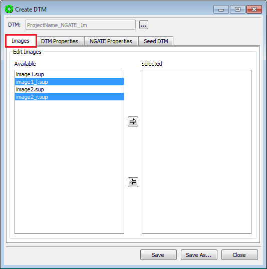
Under Edit Images, select the epipolar rectified images in the Available list and move them to Selected list via the arrow button. (The epipolar rectified images have _l and _r appended to the image name.)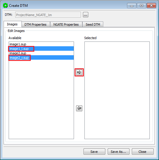

22.2.3. DTM Properties Tab

In the Create DTM window: Press the DTM Properties tab.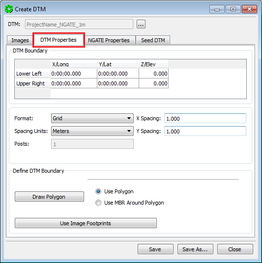
Set the X Spacing and Y Spacing to 1.0: Double click in the spacing fields, enter 1.0, and press the enter key.
Press Draw Polygon to define the DTM Boundary.
A Draw polygon window will pop-up on the stereo monitor. Move the window over to the console monitor.
Draw the polygon as follows:

a. Use the TopoMouse to define the polygon:

The Left Mouse button measures/samples points. The Right mouse button closes the polygon.

Note: the first point of the polygon will display ONLY after a second point is measured.

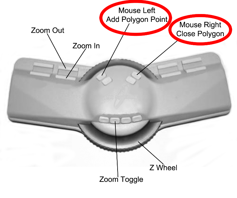
b. Make sure each DTM Boundary point is on the ground.

c. For stereo pairs of flat terrain, 4 corner points plus 2 points halfway down in the flight direction will suffice.

d. For stereo pairs of steep terrain, measure a DTM Boundary point at ‘major’ min/max elevations (i.e., at the rim of a large crater, at the crater bottom, etc.)

e. Establish the boundary within the stereo coverage by ~50 pixels. To estimate this distance:

i. Bring up the Cursor Editor (under Preferences), and change the Cursor size to 17.

ii. Move to where you want to place a boundary point.

iii. Set the image Zoom to 4:1.

iv. Aligned the cursor with the edge of the stereo coverage, then sample/measure the point.

22.2.4. NGATE Properties Tab

Press the NGATE Properties tab.
Press Strategies… to bring up the list of available NGATE strategies.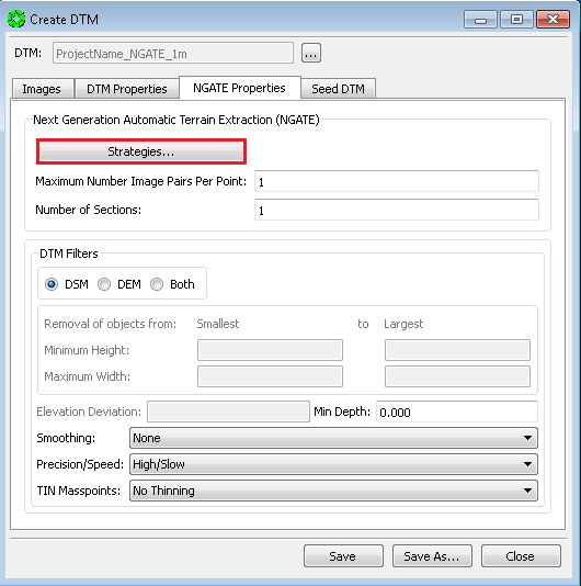
In the NGATE Strategies window, select ngate_HIRISE.strategy in the Available list and move it to Selected list via the arrow button. Then press Close.

22.2.5. Seed DTM Tab

Press the Seed DTM tab.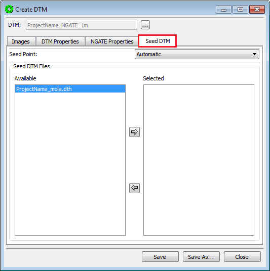
Select <ProjectName>_mola.dth in the Available list and move it to “Selected” list via the arrow button.
An error message will pop-up to change the AUTOMATIC_RSET value. Press OK.
Left-Click on the down arrow next to the Automatic option to display a drop-down box of options and select RSET64.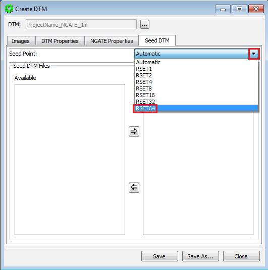
Finally, press Save to write an initialized DTM to disk. The Create DTM window will automatically close.

22.2.6. Run NGATE

NOTE: NGATE will take hours to run when extracting a DTM of the entire HiRISE stereo model. For Guest Facility Users, or others, doing production work, see Appendix: A 5.2 NGATE and AATE Batch Processing for how to run NGATE in batch.

Press Start on the NGATE window.
Upon completion of NGATE, select File > Exit.

22.3. Convert NGATE DTM to AATE format

22.3.1. Copy/Save NGATE DTM using Interactive Terrain Edit (ITE)

From the SOCET SET menu bar, select Extraction > Terrain > Interactive Edit.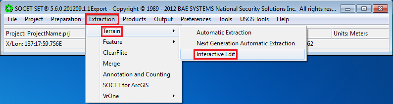
Open the newly created NGATE DTM:

a. Press the Open DTM icon in the ITE window to bring up the selection window.

b. Select <ProjectName_NGATE_1m from the DTM list. Then press OK.
On the ITE window, Select File > Save DTM As…`.
In the selection window, hand enter the name of the output DTM as <ProjectName>_AATE_onepassAfterNGATE_1m. Then press OK.
On the ITE window, select File > Exit.

22.3.2. Update AATE Header File

Edit <ProjectName>_AATE_onepassAfterNGATE_1m.dth to convert it to AATE format. (This is the DTM header file, located in the project’s data folder/directory.)

Bring up Windows/File Explorer.
Navigate to D:\\DATA\\<ProjectName>. Right-Click on <ProjectName>_AATE_onepassAfterNGATE_1m.dth and select a text editor. At USGS, use SciTE editor.
Make the following Edits:

a. Set ATE_METHOD to ADAPTIVE.

b. Delete ATE_STRATEGIES line.

c. Delete ATE_SEED_DTMs line.

d. Set MATCH_OPTION to DOUBLE_MATCH.
Select File > Save.
Select File > Exit.
Close the Windows/File Explorer window.

22.4. Replace strategy file for AATE

Replace adapt.strat with adapt.strat.onepassAfterNGATE.strat in the <install_path>\\internal_dbs\\DTM_STRATEGY folder:

Bring up a Windows Explorer window.
Navigate to C:\\SocetSet_5.6.0\\internal_dbs\\DTM_STRATEGY.
Right-Click on adapt.strat and select Delete.
Right-Click on adapt.strat.onepassAfterNGATE.strat and select Copy.
Right-Click within the folder and select Paste.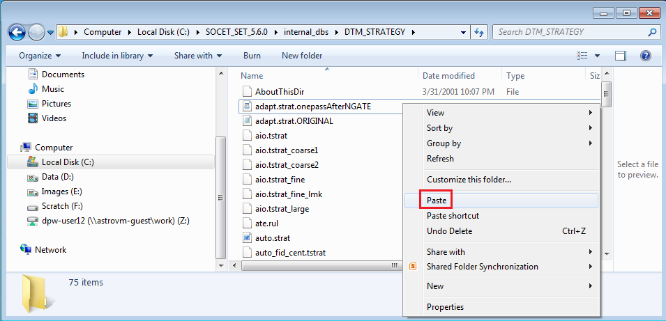
Right-Click on adapt.strat – Copy.onepassAfterNGATE and select Rename.
Rename the file adapt.strat.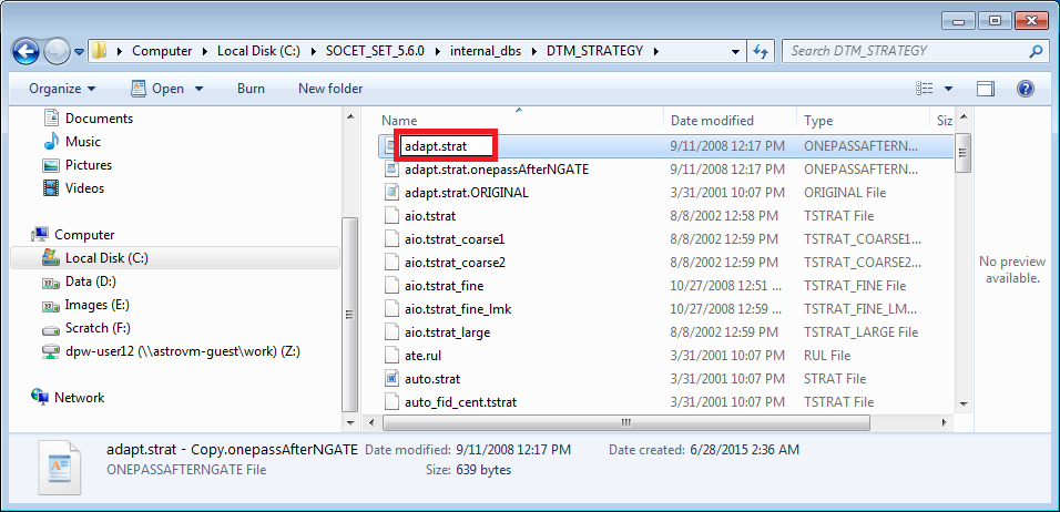
Confirm change in extension (press Yes).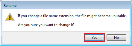
Close Windows/File Explorer window.

22.5. Adaptive Automatic Terrain Extraction (AATE)

From the SOCET SET menu bar, select Extraction > Terrain > Automatic Extraction.

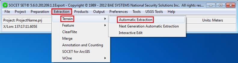
###22.5.1. Load NGATE DTM for AATE process

From the AATE window, select File > Open DTM….
Select <ProjectName>_AATE_onepassAfterNGATE_1m in the selection window. Then press OK.

22.5.2. Run AATE

NOTE: AATE can take approximately one to two hours to run when using the “onepassAfterNGATE” strategy. For Guest Facility Users, or others, doing production work, see Appendix: A 5.2 NGATE and AATE Batch Processing for how to run AATE in batch**.**

Press Start on the AATE window.
Upon completion of AATE, select File > Exit.

#23. Edit DTM

Use Interactive Terrain Edit (ITE) to display and edit DTMs. ITE provides post (point), geomorphic (line), and area editing tools. The Post Editor allows post-by-post review and edit. It is used for detailed editing of small areas. The Area Editor changes all posts within an area delineated by a polygon. It is used for smoothing, plane fill, interpolation, etc. The Geomorphic editor forces a DTM to conform to breaklines such as ridges and drains, that you draw.

The scope of this section is not to show how to use all the tools, but to suggest a few that we find most useful. What follows is our training guide for ITE. It is self-contained and steps you through loading a project, loading images, stereo display options needed for editing, setting graphical display and cursor preferences, ITE options and tips, and a FAQ section.

23.1. Loading a Project

Start SOCET SET.
Open a current project: SOCET SET > File > Load Project
Select the project from the window
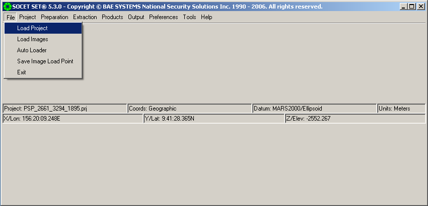
Open the Image Loader Window: SOCET SET > “File” > “Load Images”

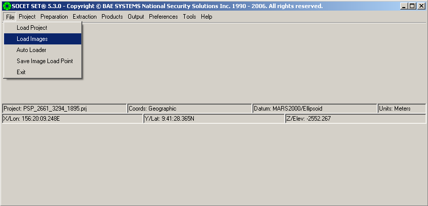
The following window will appear. Select the Left and Right Images to display. Make sure that Load Point is selected at the bottom of the window, under View Control Panel settings. Use this interface to load the epipolar rectified Left and Right images into View 1.

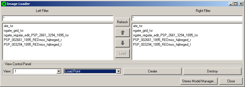
23.2. Set the stereo display, planar monitor settings

Below is an example of the settings typically used for View 1 during an editing session. (These are on the View 1 window.) The standard settings for the planar monitor, stereo display are highlighted with an arrow.

23.3. Start Interactive Terrain Edit (ITE)

Open Interactive Terrain Edit (ITE): SOCET SET > Extraction > Terrain > Interactive Edit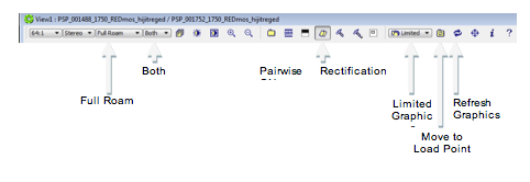
The following window will open.
Open or load the DTM with File > Open, or press the open file icon

23.4. Setting graphical display options

Open the Graphic Display Preference window for ITE: Select ITE > Options > Preferences (see Method 1). A faster, alternate method to open the Graphic Display Preference window is by clicking on the icon button toolbar along the top of the ITE Window.

23.4.1. Method 1

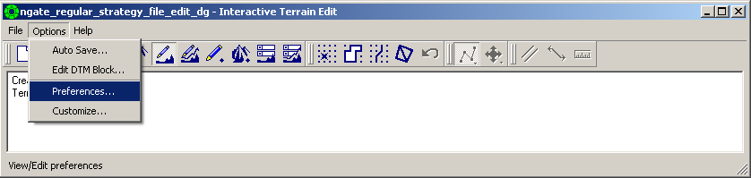
Press the Setup DTM Graphics Icon button (see Method 2)

23.4.2. Method 2

Shown below is the ITE Window toolbar.

Select the Icon shown below from the toolbar. This has the same effect as clicking on ITE > Options > Preferences

Shown below is the ITE Graphic Preferences window: The settings shown in this example are typical settings used for HiRISE DTM editing.

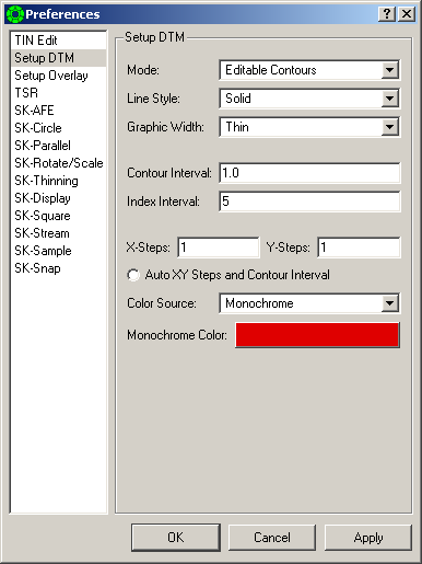
After setting your DTM graphic preferences, press the icon indicated below to draw the graphics in View 1

23.5. Setting cursor preferences

To assist in setting editing preferences, open the Cursor preference window. Select SOCET > Preferences > Cursor/Graticule Editor. Use this to save or load a cursor editor style. While editing a DTM using ITE, the cursor style keeps resetting to the default cursor style which may not be an individual user’s preferred cursor style. After setting the cursor editor style options, use File > Save Cursor to save your own style, and use File > Load to open a previously save cursor editor style.

Below is an example of a desktop, with SOCET SET/Interactive Terrain Edit initiated, and other options and preferences discussed above available.

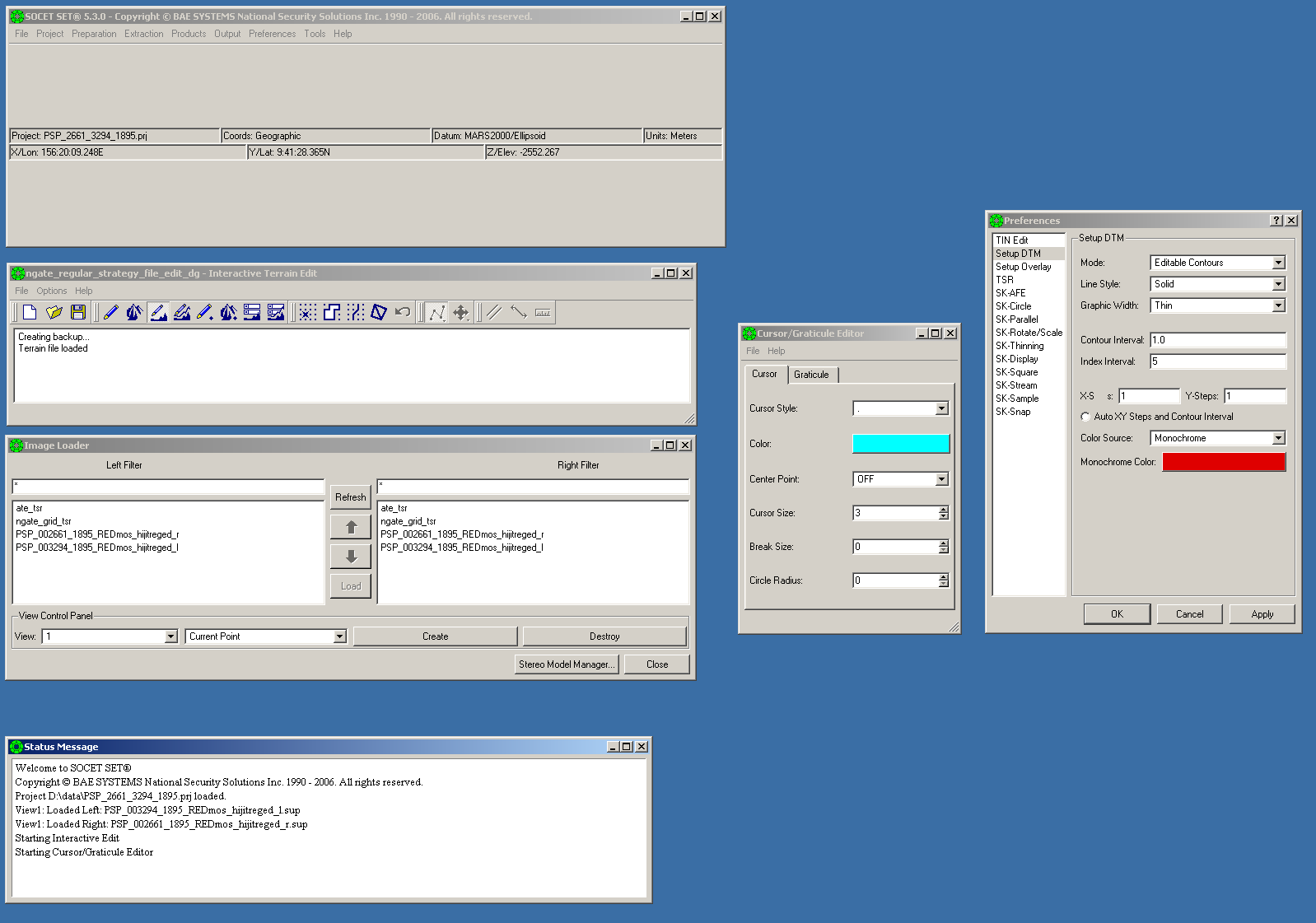
##23.6. SOCET SET Interactive Terrain Editing

Post Editing – Use this editing function when you want to adjust the elevation of the individual posts. Beware – this is a time-consuming editing choice, but it allows for high accuracy in setting individual post elevation.

Press the icon indicated below from the ITE Toolbar

The following window will open

For this editor, change the graphic display Mode (under the Preferences window) to Dots, Icons, or Editable Contours & Dots – in other words, a graphical display in which you can identify the individual posts. Click on “Grab Post” to snap to the post you want to adjust. Use the cursor arrows to move from post to post. To release the post, click again on “GRAB POST” and the cursor will release the post. Be sure to intermittently toggle the graphical display between Off/Limited at View 1 to verify that you are “on the ground”. You can also use the “snap to ground” button on the cursor to quickly move the post to ground. Visually verify that the post was moved to ground. Don’t just rely on the software.

Area Editing – Use this editing feature to adjust the elevation for a group of posts. There are many available functions within this edit feature. Below are 3 of the most commonly used.

Press the icon indicated below from the ITE Toolbar: Using the TopoMouse, draw a polygon around the area to be edited.

This area editor is great for spikes (where one or more posts are obviously off of the ground and the surrounding posts are generally on the ground). Just draw a polygon around the spike and the software will interpolate the elevation of the posts inside the polygon from those directly outside of the polygon. However, this editor rarely works against the outer edge of the DTM.

Use this area editor whenever a general smoothing of an area of post elevations is desired. It works well when the posts are generally close to the ground, but there is artificial noise. Use the “Redo” button for as many repetitions as desired. This is a good follow up to an “Interpolate_1st_order” area edit. However, if your post are “off the ground” to begin with, this area editor isn’t the best choice.

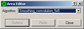This is a great area editor when it works. It systematically moves through each post within the delineated polygon and snaps it to ground. Beware! Save your edits prior to using this editor, because you cannot undo your edits – sometimes spikes are introduced! Only use this for small area edits. ITE will crash if you draw a polygon that is too large.

Geomorphic Editing – Use this editing feature to adjust the elevation for a group of posts along ridgelines, within depressions, and along slopes. It also works within crater walls and along the crater rim. With this editor, you are essentially drawing a line along the face of a feature with the goal of changing the elevation of posts within a defined (interpolation) distance on either side of the line.

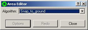
Press the icon indicated below from the ITE Toolbar:

The most commonly used Algorithm with this editor is “Uniform Slope”. Set the “Interpolation Distance” by first estimating the distance based on the resolution of the DTM to be edited (For HiRISE DTMs use 1 – 5 M, MER MI DTMs require a much smaller distance). Then, using trial-and-error, find the best distance for the type of feature that you are editing. Generally, along the sides of slopes, a greater Interpolation Distance works well, while along a crest or ridge line, a narrower, or smaller distance is used. Be sure to toggle between Limited/Off for the graphics display to make sure that the posts (as displayed by contours) are on the ground.

UNDO The button indicated below allows one “undo” following the execution of any edit except the “Snap_to_ground” area edit. Use this if any edit function produces unexpected and undesired results! But remember that you can only “back-up” once.

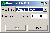
Editing Using a Triangulated Irregular Network (TIN) A special editing function is accessed by clicking on the indicated icon. This edit feature allows the user to use TIN tools to edit a delineated area within a DTM/GRID. Remember that the DTMs normally produced for editing are in a GRID format, meaning that the posts are in a regularly spaced grid pattern. A TIN is an irregularly spaced framework of posts. Unique editing tools are available once a defined area is temporarily converted into a TIN. Use this edit feature for terrain that is complicated and requires high DTM accuracy.

TIN editing mouse button functions to remember: Toggle cursor and delineate a polygon (left mouse button). Accept polygon (right mouse button) to start the area tool. Pick/Move Post = Left mouse button Delete Post = Middle mouse button New Post = Right mouse button

The first step is to click the highlighted icon. The following window will open. Draw a polygon around an area to be edited, as requested.

Once the delineated area has been converted into a TIN, the other edit functions describe above are available for use. Post editing is especially useful here. One option is to set the DTM graphic preferences to a mesh to see the posts and TIN structure easily. TIN based editing functions are flexible and powerful.

##23.7. FAQ

What should I do when it appears that the edit function I have selected isn’t doing anything?

First make sure that you closed the edit polygon (area edits) or completed your line drawn (geomorphic editor). Then make sure that the edit settings are reasonable for the DTM you are currently working on. Is the Interpolation Distance defined in the geomorphic editing window entered correctly? If everything appears to be set up correctly, close the editor and re-open it. Sometimes ITE gets “stuck” and needs to be restarted.
I can’t get ITE to open. The Menu button for ITE is grayed out and nothing happens when I click it.

Make sure that you have opened Load Images. From the Load Images window, correctly select both images, and press “Load”. ITE can’t be initialized without images loaded in View 1.

24. Generate Orthorectified Images

For HiRISE, it is useful to generate an orthoimage of each image in the stereo pair at both (a) 1 m resolution, exactly matching the DTM, and (b) 0.25 m resolution to preserve the maximum information in the images.

We use the controlled images (not the epipolar rectified images with _r and _l extensions), without enhancements, as input for orthorectification.

24.1. Move or Delete Enhancement Files

Make sure there are no image enhancement files associated with the input image in the project data directory before proceeding. Enhancement files are stored in the Project’s data folder (i.e., D:\\DATA\\<ProjectName>) and have an extension of .enh.

a. If there are enhancement files, delete them or move them somewhere else temporarily.

b. We do this because image brightness/contrast adjustments in the enhancement files will be applied to the orthorectified image upon creation. We are keeping track of the stretch to 8-bit when processing HiRISE images for SOCET SET import so that we can get back to radiometric values if needed. Appling an arbitrary stretch through enhancement files will defeat this purpose.

24.2. Run Calc Ortho Boundary

So that a 1:1 correspondence between the DTM and the 1 m orthoimages is maintained in software packages such as ISIS and Photoshop, we run “calc Ortho Boundary” to calculate Lower Left and Upper Right georeferencing corner coordinates to be used as input for orthophoto generation.

From the SOCET SET menu bar, select USGS Tools > Calc Ortho Boundary.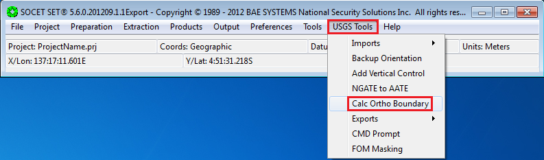
If the project file listed in the Project File field is correct, check the box next to the Project File field to confirm it. Otherwise, press the Project File… button to bring up the list of projects and select the project from the list.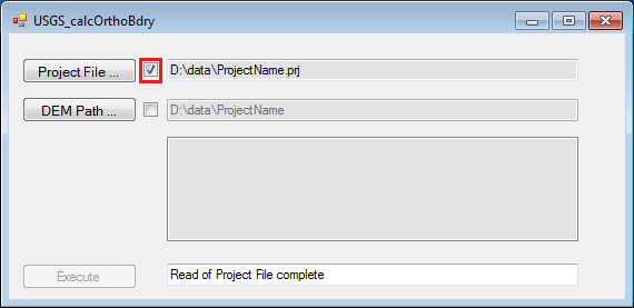
The path listed in the DEM Path field should be the path to the current project’s data folder. If the path is correct, check the box next to the DEM Path field to confirm it. Otherwise, press DEM Path…, and navigate to the project’s data folder to select it.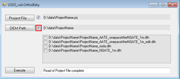
Upon confirming the DEM Path, the available DTMs in the project will be listed. Select the final edited version of the DTM by clicking on its check box twice. Then press Execute.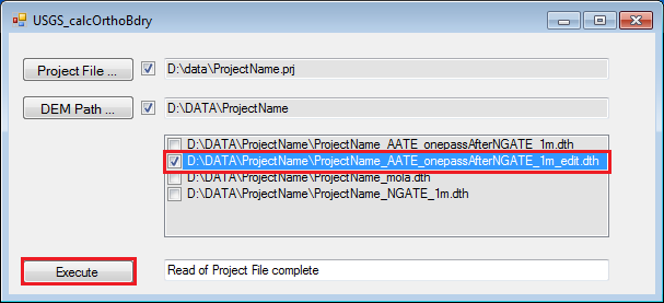
Close the Command Prompt Window that came up.
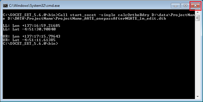
The results of Calc Ortho Boundary is written to a log file in the project’s data folder. The log name is of the form calcOrthoBdry_<the_input_DTM_name>.log.

24.3. Orthophoto Generation

Note: Generation of 1 m orthoimages takes 1 to 2 hours. Generation of 0.25 m orthoimages can take up to 12 hours each. (These time estimates are based on the current processors configuration at the Planetary Photogrammetry Facility.) For Guest Facility Users or Astrogeology staff, doing production work, see Appendix: A-5.3 Orthophoto GenerationBatch Processing for how to run Orthophoto in batch.

From the SOCET SET menu bar, select Products > Orthophoto Generation.

24.3.1. Start Tab

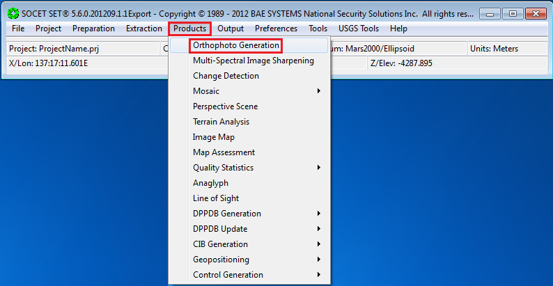
In the Start Tab, make sure Task is set to Orthphoto.

24.3.2. Input Tab

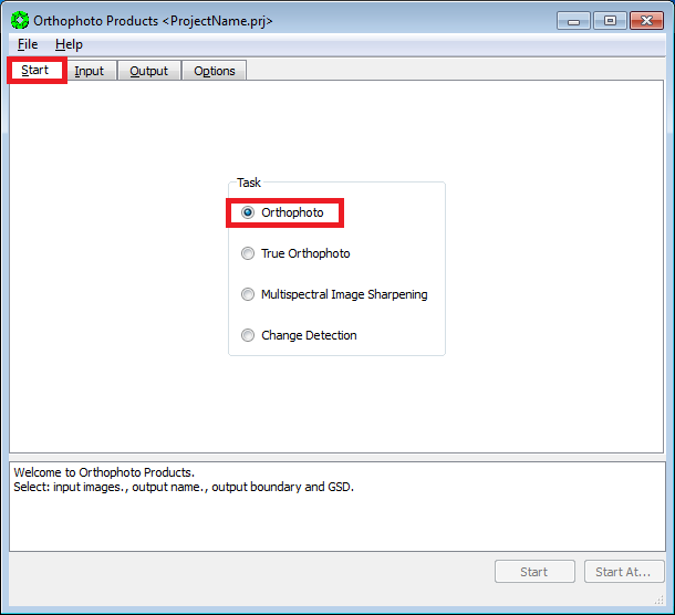
Press the Input tab.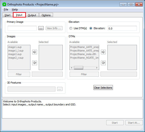
Press the button next to the Primary Image field.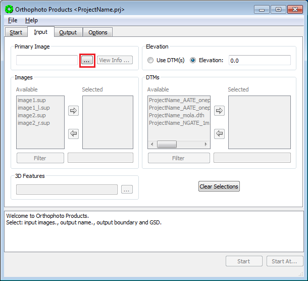
In the pop-up window, select the image to orthorectify. Then press OK. Do not select the epipolar rectified images.
Press the radio button for Use DTM. Then, from the list of Available DTMs, move the final (edited) DTM to the Selected list via the arrow button.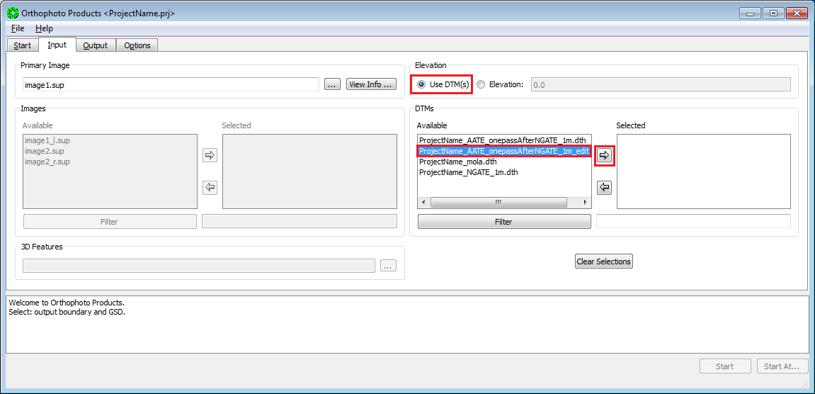

24.3.3. Output Tab

Press the Output tab.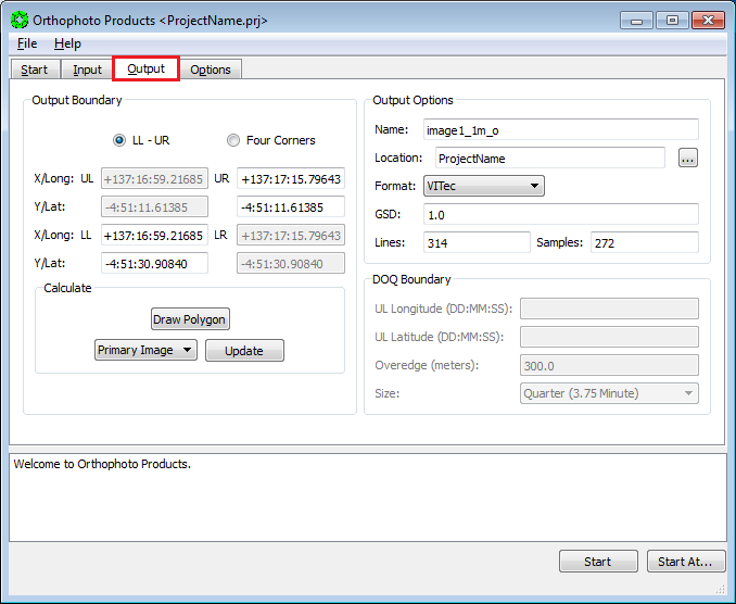
Bring up a Windows/File Explorer window. Navigate to D:\\DATA\\<ProjectName> and open calcOrthoBdry_<DTMname>.log with a text editor.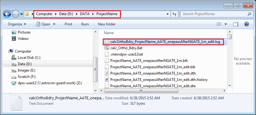
In the Output Boundary Section of the Orthophoto window:

a. Turn on radio button LL-UR in the Output Boundary section.

b. Then copy-and-paste the LL and UR coordinates from calcOrthoBdry_<DTMname>.log into the LL and UR boxes. Do not press “Update” after entering LL and UR coordinates.

Note: You only need to copy-and-paste the LL and UR coordinates once…the values will hold for multiple orthophoto setups.
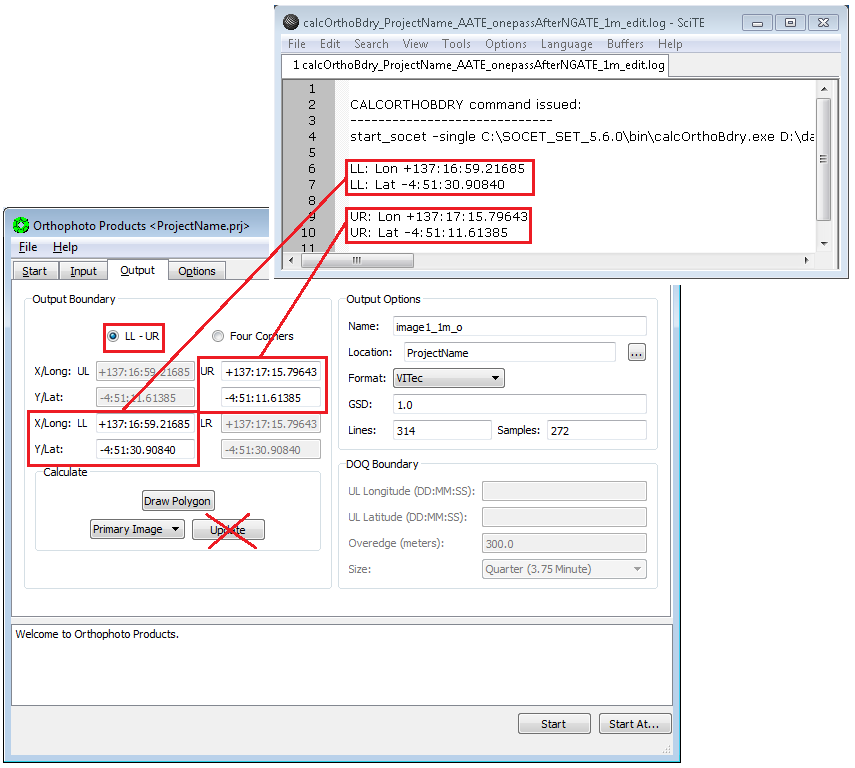
In the Output Options Section:

a.  Change the default `Name` of the orthoimage from
    `<image>_o` to `<image>_1m_o` or
    `<image>_25cm_o`, as appropriate.

b.  Make sure the `Location` is set to the project’s image location,

c.  Use the drop down arrow to set `Format` to Vitec.

> Note: We’ve had problems with TIFF-Tiled format when
    orthorectifying large images.

d.  Type in the `GSD` (ground sample distance) of the desired
    resolution (e.g., 1 m or 0.25 m). Then press the enter key.

   	![](media/image486.png)

24.3.4. Options Tab

Press the Options tab.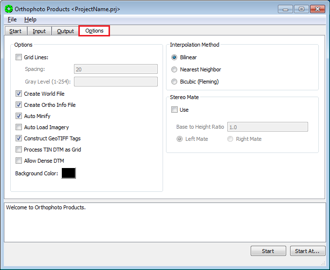
In the Options Section:

a. Check the boxes for:

i. Create World File.

ii. Create Ortho Info File.

iii. Auto Minify.

b. Set the Background Color to Black: Click on box displaying background color to cycle through color options.

24.3.5. Run Orthophoto

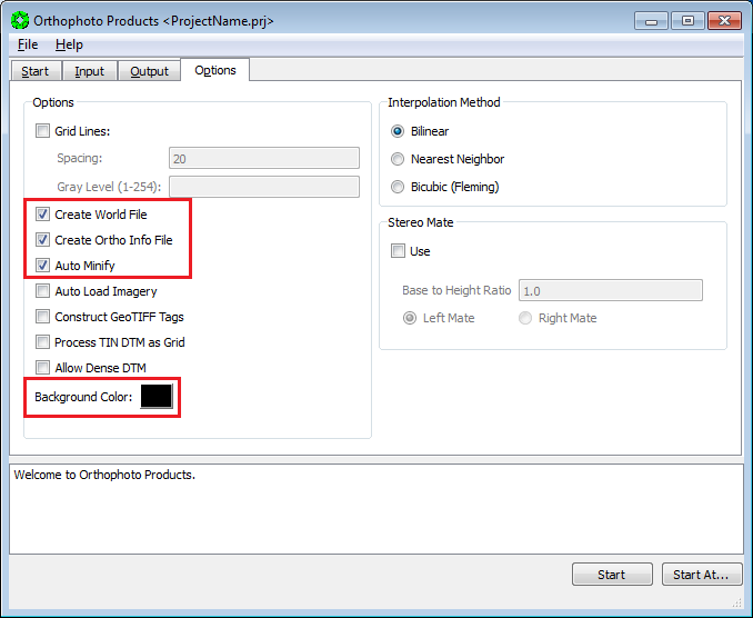
Press Start at the bottom of the Orthophoto window.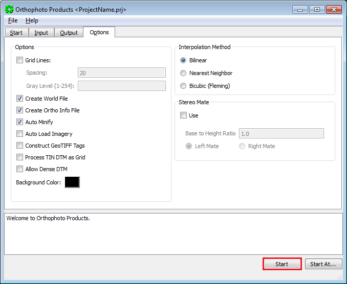
Go To 23.3.2 Orthophoto Generation, and repeat the steps for next orthoimage.
Close the Orthophoto Products window when all orthoimages are generated.

#25. Export DTMs and Orthoimages

25.1. Brief Overview

Exporting DTMs and Orthoimages is a two step process:

First we run utilities/programs on the SOCET SET workstations to convert SOCET SET file formats to raw binary files and build corresponding ISIS3 scripts. All raw binary files and ISIS3 scripts are placed in folder D:\\DATA\\<ProjectName>\\Output_Products.
Then we copy the entire D:\\DATA\\<ProjectName>\\Output_Products folder to an ISIS3 processing machine, where the scripts are executed to generate the ISIS3 cubes.

25.2. Export DTMs

From the SOCET Set menu bar, select USGS Tools > Exports > Export DEM to ISIS.
Press Project File.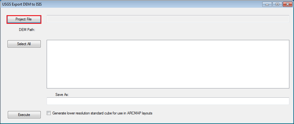
In the Open window, navigate to the main SOCET SET DATA folder (D:\\DATA), select file <ProjectName>.prj, and then press “Open”.
Select DTM(s) to export. Either:

a. Press Select All if you wish to export all DTMs, or

b. Double click on the check box for each DTM you wish to export.
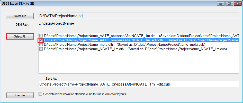
Press Execute.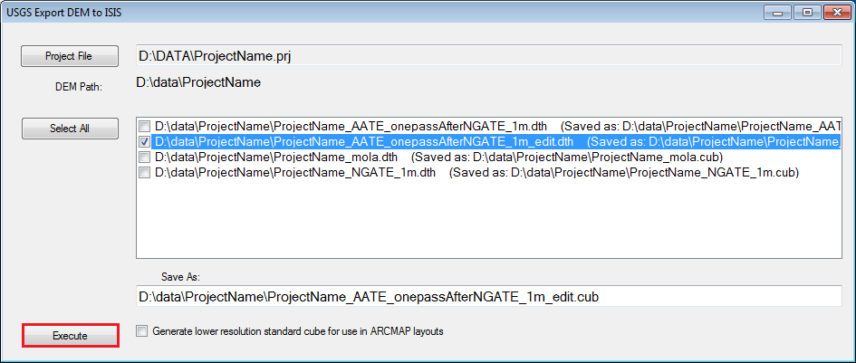
A Command Prompt window will pop-up. Upon completion of the program, close the Command Prompt window.

25.3. Export Orthoimage(s)

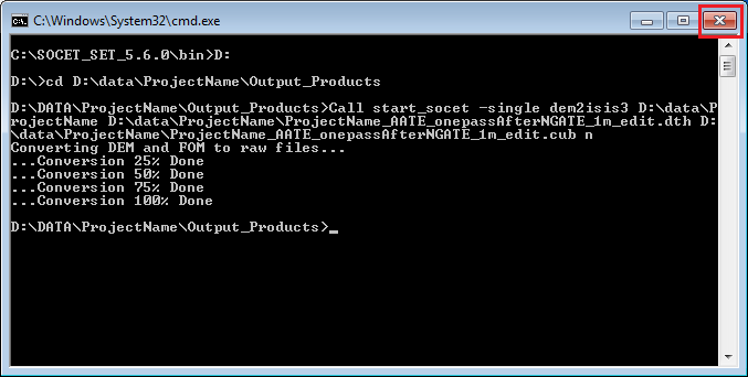
From the SOCET Set menu bar, select USGS Tools > Exports > Export Orthos to ISIS.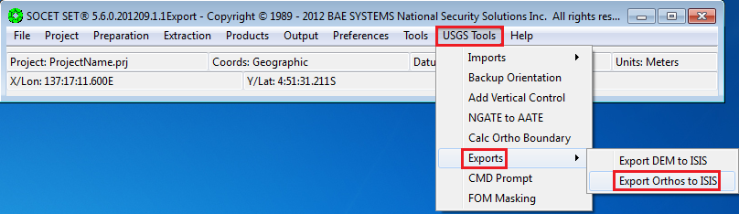
Press Project File.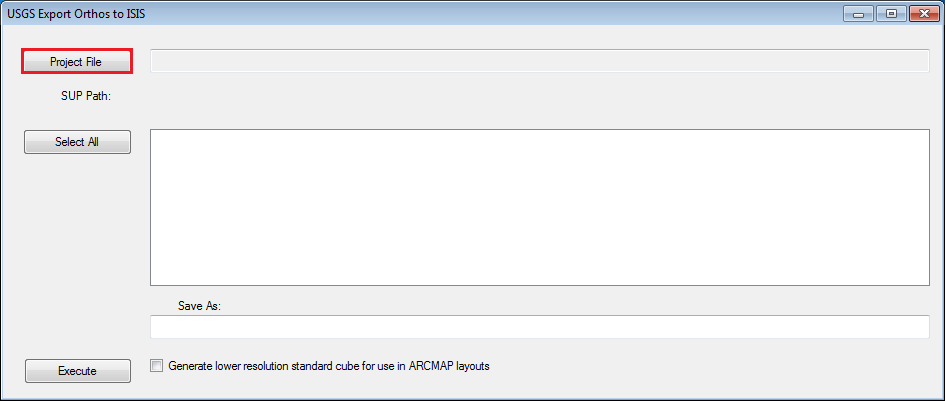
In the Open window, navigate to the main SOCET SET DATA folder (D:\DATA), select file .prj, and then press Open.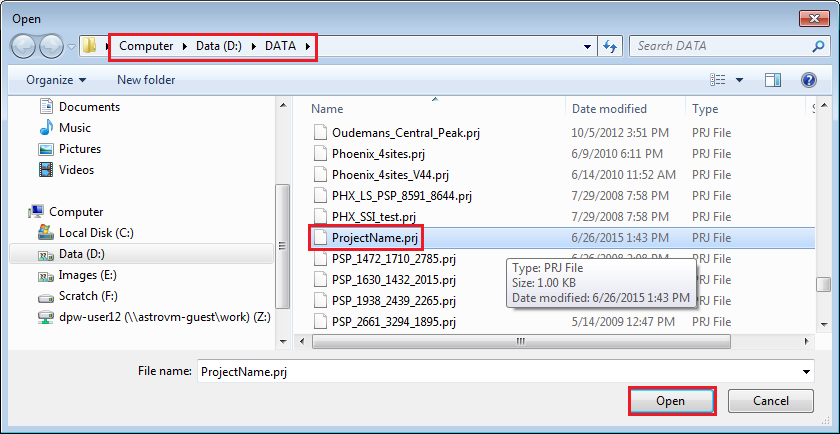
Select Orthoimages to export (these will have the _o suffix): double click on the check box for each Orthoimage you wish to export.
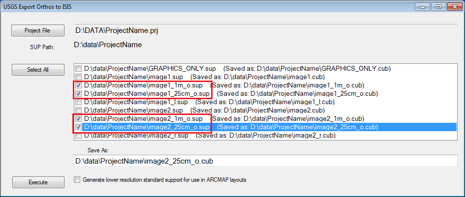
Press Execute.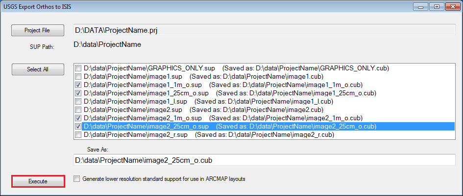
A Command Prompt window will pop-up. Upon completion of the program, close the Command Prompt window.

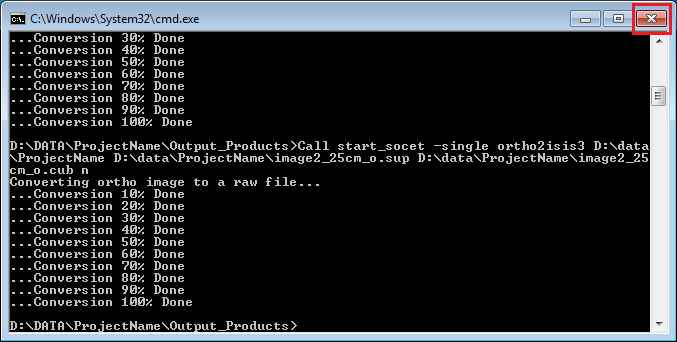
25.4. Transfer Files to ISIS Processing Machine

Using Windows/File Explorer, copy the <data_path>\\<ProjectName>\\Output_Products folder to a shared network drive. Place Output_Products in the <ProjectName> working directory/folder on the ISIS machine.

25.4.1. File Transfer for USGS Astrogeology Guest Facility Users

Bring up Windows Explorer and navigate to D:\\DATA\\<ProjectName>.
Bring up a second Window Explorer window, and navigate to Z:\\<ProjectName>.
Copy the entire Output_Products folder from D:\\DATA\\<ProjectName> to Z:\\<ProjectName>.

25.5. Generate ISIS3 Cubes

Log onto the ISIS Processing (UNIX) Machine. For Guest Facility Users, log onto astrovm-guest (see 1 Guest Facility Log On Procedure for details.)
In the Unix window, change directory into the <ProjectName>/Output_Products directory.

Unix Command for Guest Facility Users is:
```
$ cd <ProjectName>/Output_Products
```
Unix Command for Astro Employees is:
```
$ cd <path_to_ProjectName>/Output_Products
```
Run dos2unix on the scripts to update linefeed/carriage-return differences between Windows and UNIX. Use the wildcard (*) to update all scripts with one command, as follows:
```
$ dos2unix \*.sh
```
Run setisis to initiate ISIS, as follows:
```
$ setisis isis3
```
Use the source command to execute each script. Wildcarding does not work with source, so use awk to generate a script to source all the dem- and ortho-to-isis scripts “automatically. The commands are:
```
$ ls \*.sh | awk ‘{print “source”,\$1}’ > generate_cubes.script
$ source generate\_cubes.script<a name="conversionofisis3cubetoarccompatibleformats"></a>
```

26. Conversion of ISIS3 Cube to ARC Compatible Formats

26.1. Coordinate System Compatibility Requirements for ArcMap

For Mars: when working in a Geographic project, the native SOCET SET files are in the ographic latitude, +E longitude system. To use the most widely used coordinate system for Mars (East longitude and planetocentric latitude), use the standard ISIS3 cubes exported from SOCET SET (not the cubes with the SS_ prefix)
ArcMap expects positive East longitude coordinates, but some planetary bodies have positive West longitude definitions as per the IAU. The SOCET SET to ISIS export software maintains the IAU standards on longitude direction. To insure ArcMap 10+ will ingest both positive East or positive West defined cubes correctly, the CENTER_LONGITUDE on the ISIS cubes are set to 0.0.

Geographic projects in SOCET SET produce Equi-Rectangular map projected DTMs and Orthoimages. For the Equi-Rectangular map projection, changing the CENTER_LONGITUDE value will not require a resampling of the DTMs and Orthoimages. It only translates the x-coordinates of the Equi-Rectangular map projection coordinates.

26.2. ISIS3 Cubes Compatible with ArcMap 10+

The good news is that ArcMap version 10+ will directly load ISIS3 map-projected cubes, so conversion of file formats is no longer required!

26.3. Conversion to GeoTiff

SOCET Set has an export tool to output DTMs and images as GeoTiff images, however, it does not cover planetary images correctly (the GeoTiff header out of SOCET SET is incomplete.)

To generate GeoTiff images and DTMs, start with the ISIS3 cube as input, and run hi_isis2geotiff.pl as follows:

To convert an ortho image, enter the following on the command line:

$ hi_isis2geotiff.pl -ortho <ortho.cub>;
To convert a DTM, enter the following on the command line:

$ hi_isis2geotiff.pl -dem <DTM.cub>

26.4. Conversion to JP2

To convert ISIS3 Orthoimage (8 bit cube) to 8-bit JPEG 2000 file: only one extension is allowed in the input cube name (this is a GDAL PCI Aux format issue), so if two extensions exist e.g., PSP_00XXXX_XXXX_1m_o.isis3.cub, then

First rename the cube as follows:

$ mv <image_id>_1m_o.isis3.cub <image_id>_1m_o_isis3.cub
Then run isis3gdal_jp2.pl as follows:

$ isis3gdal_jp2.pl .cub .jp2

Parameter	Accuracy
IT pos. bias	100 m
CT pos. bias	100 m
Radial pos. bias	10 m
IT vel. bias	13 m/s
CT vel. bias	13 m/s
Radial vel. bias	1.3 m/s
Kappa bias	0.1 degree