Mesh Reconstruction
- Mesh Reconstruction Panel
- Reconstruction Methods
- Colors and Materials Options
- Meshing Options
- Spines Options
- Rendering Options
- Navigation
This panel gives access to the parameters of the Meshing toolbox. This toolbox is used to reconstruct polygonal mesh models - a collection of vertices, edges and faces that represent the shape of a polyhedral object in the three-dimensional space - that reflect the membrane surface of the neurons from their morphological skeletons.
When all the meshing parameters are set, a neuronal mesh can be reconstructed by clicking on the button Reconstruct Mesh. Once the mesh is reconstructed, it will appear in the principal three-dimensional view port of Blender. The mesh can be then rendered to image by clicking on the different views buttons: Front, Side, or Top. We can also render a 360 movie of the reconstructed mesh by clicking on the 360 button. Finally, the mesh can be exported to different file formats such as .obj, .ply, .stl and .blend meshes.


The current version of NeuroMorphoVis implements four different meshing algorithms:
- Piecewise Watertight Meshing
- Skinning-based Meshing
- Union-operator-based Meshing
- MetaBalls Meshing
- Voxelization-based Remeshing

The piecewise wateright meshing is proposed by Abdellah et al, 2017. This method reconstructs a single mesh object that is composed of a set of watertight meshes, each corresponding to an individual component in the original morphology skeleton. For example, breadth-first traversal is used to connect and construct primary sections along each arbor in the form of tubes. These tubes are converted into watertight meshes that by definition have non-manifold edges or vertices. The grouping of the reconstructed meshes results in the final mesh object that is not watertight per se, but rather piecewise-watertight.
Further details about this meshing technique is available in this page.


This technique can be set in the configuration file as follows:
# Meshing technique
MESHING_TECHNIQUE=piecewise-watertightThis method generates high fidelity surface meshes of neurons from their morphological skeletons using the Skin Modifier in Blender. The Skin modifier uses vertices and edges to create a skinned surface, using a per-vertex radius to better define the shape. The output is mostly quads, although some triangles will appear around intersections. It is a quick way to generate base meshes for sculpting and/or smooth organic shapes with arbitrary topology. For further details on the approach and the implementation, please refer to the full publication by Abdellah et al., 2019.


This technique can be set in the configuration file as follows:
# Meshing technique
MESHING_TECHNIQUE=skinningThe union-operaator-based meshing is similar to the piecewise watertight meshing technique. This approach uses union operators to merge the different meshes into a single object without being intersecting.
The following rendering shows a comparison between two meshes reconstructed with the piecewise-watertight and union-operator techniques. Notice how the overlapping between the different sections in the first technique is resolved by the applying the union operators to each two connected components in the mesh produced by the piecewise watertight meshing.


This technique can be set in the configuration file as follows:
# Meshing technique
MESHING_TECHNIQUE=union

In general, Meta objects are implicit surfaces, meaning that they are not explicitly defined by vertices (as meshes are) or control points (as surfaces are): they exist procedurally. The fundamental feature that makes meta objects significant is their ability to blend, i.e. when two independent meta objects are getting closer to each other, they start to interact and blend together into a single object. This algorithm is capable of handling highly complex branching scenarios avoiding to create intersecting geometry that is common in other meshing algorithms, for example skinning with skin modifiers. In this algorithm, we build a meta object of the neuron morphology using meta balls and convert it to a mesh in the final stage. The resulting mesh is guaranteed to be two-manifold, but it might contain self intersections based on the meta resolution used to convert the meta object into a mesh.


Further details about this meshing technique is available in this page.
This technique can be set in the configuration file as follows:
# Meshing technique
MESHING_TECHNIQUE=meta-balls
Normally, meshes created with the MetaBalls algorithm have high polygon counts and bumpy effects. Therefore, it is advisable to use the tessellation option to reduce the number of polygons in the final mesh and remove these bumps. This is shown in the following comparison.


In the recent versions of Blender (3.0 and above), voxelization-based remeshing modifiers were integrated. We therefore built upon this integration and implemented a voxelization-based remeshing modifier that can create watertight meshes of any input morphologies irrespective their geometric complexity. The implementation uses either the piecewise-watertight meshing or the articulated sections morphology builder to reconstruct proxy geometries that can be used with the remeshing modifier to create the final watertight mesh. Note that the surface of the resulting mesh will have a single color.

This technique can be set in the configuration file as follows:
# Meshing technique
MESHING_TECHNIQUE=voxelizationResulting meshes can be optimized based on the OMesh library. Further instructions on this library can be found in this page.
Users can assign multipl shaders or materials to the different compartments of the mesh. This includes:
- Soma Color
- Axon Color
- Basal Dendrites Color
- Apical Dendrite Color
- Spines Color (optional if the spines are generated)
All available shaders in NeuroMorphoVis are demonstrated in this page.

Depending on the meshing technique, users can either assign different colors to the different components (soma, axon, apical dendrite, basal dendrites and spines) of the mesh or use a homogeneous color to be applied to the entire mesh.

This color options can be set in the configuration file as follows:
# Soma RGB color in the form of normalized 'R_G_B' tuple
SOMA_COLOR='1.0_1.0_0.0'

# Axon RGB color in the form of normalized 'R_G_B' tuple
AXON_COLOR='0.0_0.0_1.0'

# Basal dendrites RGB color in the form of normalized 'R_G_B' tuple
BASAL_DENDRITES_COLOR='1.0_0.0_0.0'

# Apical dendrite RGB color in the form of normalized 'R_G_B' tuple
APICAL_DENDRITE_COLOR='0.0_1.0_0.0'

# Spines RGB color in the form of normalized 'R_G_B' tuple
SPINES_COLOR='1.0_1.0_0.5'
If the Union, MetaBalls and Voxelization techniques are selected, users can only assign a single color to the entire mesh from the Membrane Color field.
In this case, this unique color can be set in the configuration file from the SOMA_COLOR as follows:
# Soma RGB color in the form of normalized 'R_G_B' tuple
SOMA_COLOR='1.0_1.0_0.0'- MetaBalls
- SoftBody
The soma surface is generated with the MetaBalls algorithm. This approach is almost instantaneous.
This option can be set in the configuration file as follows:
# Soma method
SOMA_METHOD=meta-ballsThe soma surface is generated with the SoftBody simulation. This approach is a little bit time consuming. It might take few seconds to reconstruct the soma depending on the complexity of the arborization.

This option can be set in the configuration file as follows:
# Soma method
SOMA_METHOD=soft-body- Sharp
- Curvy
The edges between the segments are sharp like a piece-wise linear function.

This option can be set in the configuration file as follows:
# Edges
EDGES=hardThe edges along each branch are smoothed to look curvy.

This option can be set in the configuration file as follows:
# Edges
EDGES=smooth- Smooth
- Rough
The surface of the mesh is clean.
This option can be set in the configuration file as follows:
# Surface
SURFACE=smoothThe surface of the mesh has perturbations to reflect neurons reconstructed from electron microscopy (EM) stacks. This option is only valid when the Curvy edges option is selected.

This option can be set in the configuration file as follows:
# Surface
SURFACE=rough- Connected
- Disconnected
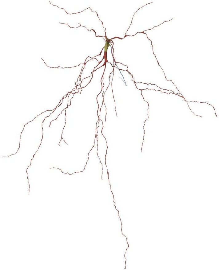
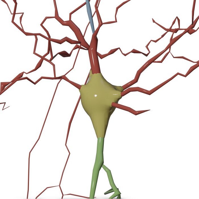
The soma mesh is connected to arbors to in a continuous form. With this approach, there are no artifacts along the connections between the soma and the arbors.

The soma mesh is actually disconnected from the arbors, but logically added at the center. Users might notice some minor artifacts between the soma and the arbors. Notice the connection between the apical dendrite in green and the soma in yellow in the following image. Compare this to the previous one.

- Connected
- Disconnected
All the different mesh objects are connected or joint together with a joint operation.

Every mesh object is independent and can be exported as an individual mesh. This option is used to tag the different compartments of the neuron in other applications.

We added an option to allow controlling the tessellation level of the mesh in case the mesh has too many polygons. If checked, this option will apply a tessellation modifier on the mesh to reduce the number of polygons in the mesh. To contro the tessellation, you can select the tessellation factor from the Factor slider. The acceptable range of this parameter is 0.99 and 0.1.

Users can integrate spines along the mesh surface.
Ignore adding spines.
Add random spines if the neuron is not loaded from a circuit to be able to detect the pre-post synaptic connectivity with other cells. Users can control the quantity of the spines from the Percentage slider.

If a neuron is loaded from a BBP circuit, then users can get the locations of the actual spines that are reported in the circuit. This option will not appear in the GUI if the neuron is not loaded with a specific GID from a specific circuit.
Use high quality spines. This option is only recommended for high quality media generation of close up views becuase it will take time to load the spines in the scene.
Use low quality spines. This option is recommended for overall views of the neuron from a far away distance.
Similar to rendering morphologies, users can render the following shots of the mesh:
- Wide Shot
- Mid Shot
- Close Up
To understand the difference between the different shots in general, you can refer to this artlcie.
The spatial extent of a wide shot image spans that of the entire morphology, even if we limit the branching order to certain level. To render a wide shot view of the mesh, the option Wide Shot must be selected before clicking on any rendering button.


This option can be set in the configuration file as follows:
# Rendering view
RENDERING_VIEW=wide-shotThe spatial extent of a mid shot image is limited to the bounding box of only the arbors reconstructed at a specific branching order. To render a mid shot view of the mesh, the option Mid Shot must be selected before clicking on any rendering button.


This option can be set in the configuration file as follows:
# Rendering view
RENDERING_VIEW=mid-shotIf you select to render a closeup view of the mesh (around the soma) by clicking on the Close Up button, then you can set the size of the closeup shot in the Close Up Size field.

This option can be set in the configuration file as follows:
# Rendering view
RENDERING_VIEW=close-up

# Close up view dimensions (in microns)
CLOSE_UP_VIEW_DIMENSIONS=20NeuroMorphoVis has support to set the resolution of the rendered images either to a fixed resolution or based on the dimensions of the morphology skeleton. The later option is mandatory for images required for scientific articles. It allows users to render images to scale and overlay a scale bar on the top of the image.
The resolution of the image is defined by two parameters (width and height) in pixels, however, NeuroMorphoVis forces the users to define the resolution of the image using a single parameter to avoid rendering an image with distrorted aspect ratio.
This option can be set in the configuration file as follows:
# Renders a frame to scale
RENDER_TO_SCALE=no


# Frame resolution, only used if RENDER_TO_SCALE is set to no
FULL_VIEW_FRAME_RESOLUTION=4000Before rendering the reconstructed mesh into an image, the three-dimensional bounding box (width, height and depth) of the mesh is automatically computed and the resolution of the image is defined based on 1) the bounding box of the mesh and 2) the rendering view. For example if the bounding box of the mesh is 100 x 200 x 300 and a front view is rendered, then the resolution of the image will be set automatically set to 100 x 200. If the side view of the mesh is rendered, then the resolution of the image will be set to 200 x 300 and finally if the top view is rendered, then the resolution of the image will be set to 300 x 100. If the user wants to render an image to scale, then option To Scale must be selected. In this case, each pixel will correspond in the image to 1 micron, and the resolution of the image is limited to the dimensions of the morphology. To render higher resolution images, however to scale, we have addedd support to scale the resolution of the image using a scale factor that is defined by the user. When the user select the To Scale option, the Scale Factor slider appears below to give the user the control to select the most approriate scale factor that fits the objective ultimate objectives of the image. By default, the scale factor is set to 1. Note that increasing the scale factor will make the rendering process taking longer O(NXM). A convenient range for the scale factor is 3-5.

This option can be set in the configuration file as follows:
# Renders a frame to scale
RENDER_TO_SCALE=yes

# Frame scale factor (only in case of RENDER_TO_SCALE is set to yes), default 1.0
FULL_VIEW_SCALE_FACTOR=10.0Users can render the following camera views of the morphology:
- Front
- Side
- Top

This option can be set in the configuration file as follows:
# Camera view
CAMERA_VIEW=frontNeuroMorphoVis can render 360 sequences for the reconstructed meshes.
This option can be set in the configuration file as follows:
# Render a 360 sequence of the mesh, default 'no'.
# Use ['yes' or 'no']
RENDER_NEURON_MORPHOLOGY_360=yesUsers can exploit the native support of Blender to export meshes into different file formats. But since we assumed that end users might not have any Blender experience, we have added explicit support to allow them exporitng the reconstructed meshes into the following common file formats:
-
Wavefront (.obj) The OBJ file format is a simple data-format that represents 3D geometry alone — namely, the position of each vertex, the UV position of each texture coordinate vertex, vertex normals, and the faces that make each polygon defined as a list of vertices, and texture vertices. Further details about this file format can be found here.
-
Stanford (.ply) PLY is a file format known as the Polygon File Format or the Stanford Triangle Format. It was principally designed to store three-dimensional data from 3D scanners. The data storage format supports a relatively simple description of a single object as a list of nominally flat polygons. A variety of properties can be stored, including: color and transparency, surface normals, texture coordinates and data confidence values. The format permits one to have different properties for the front and back of a polygon. Further details about this file format can be found here.
-
Stereolithography CAD (.stl) The STL file describes a raw, unstructured triangulated surface by the unit normal and vertices (ordered by the right-hand rule) of the triangles using a three-dimensional Cartesian coordinate system. Further details about this file format can be found here.
-
Blender Format (.blend) The exported file can be opened only in Blender and can be used for rendereing purposes.
The exported meshes will be generated in the meshes directory underneath the output directory that is set by the user in the Input / Output panel.
Note If this path is not set, the user will get this error message Output directory is not set, update it in the Input / Output Data panel. In this case, the user must toggle the Input / Ouput panel and update the Output Directory by replacing Select Directory in the output options by an existing path on the file system.
These options can be set in the configuration file as follows:
# Export .PLY meshes
# Use ['yes' or 'no']
EXPORT_NEURON_MESH_PLY=no

# Save .OBJ meshes
# Use ['yes' or 'no']
EXPORT_NEURON_MESH_OBJ=no

# Save .STL meshes
# Use ['yes' or 'no']
EXPORT_NEURON_MESH_STL=no

# Export the mesh in a .BLEND file
# Use ['yes' or 'no']
EXPORT_NEURON_MESH_BLEND=no

# Export each part (or component) of the mesh as a separate file for tagging
# Use ['yes' or 'no']
EXPORT_INDIVIDUALS=no-
Abdellah et al. "Generating high fidelity surface meshes of neocortical neurons using skin modifiers." EGUK Computer Graphics and Visual Computing Proceedings (2019).
-
Abdellah et al. "NeuroMorphoVis: a collaborative framework for analysis and visualization of neuronal morphology skeletons reconstructed from microscopy stacks." Bioinformatics 34.13 (2018): i574-i582.
-
Abdellah et al. "Reconstruction and visualization of large-scale volumetric models of neocortical circuits for physically-plausible in silico optical studies." BMC bioinformatics 18.10 (2017): 402.
-
Lasserre et al. "A neuron membrane mesh representation for visualization of electrophysiological simulations." IEEE Transactions on Visualization and Computer Graphics 18.2 (2012): 214-227.
-
Blender documentation, MetaBalls.
-
Starting
-
Panels
-
Other Links
![]()
![]()