Simple Systematic Point Simulation

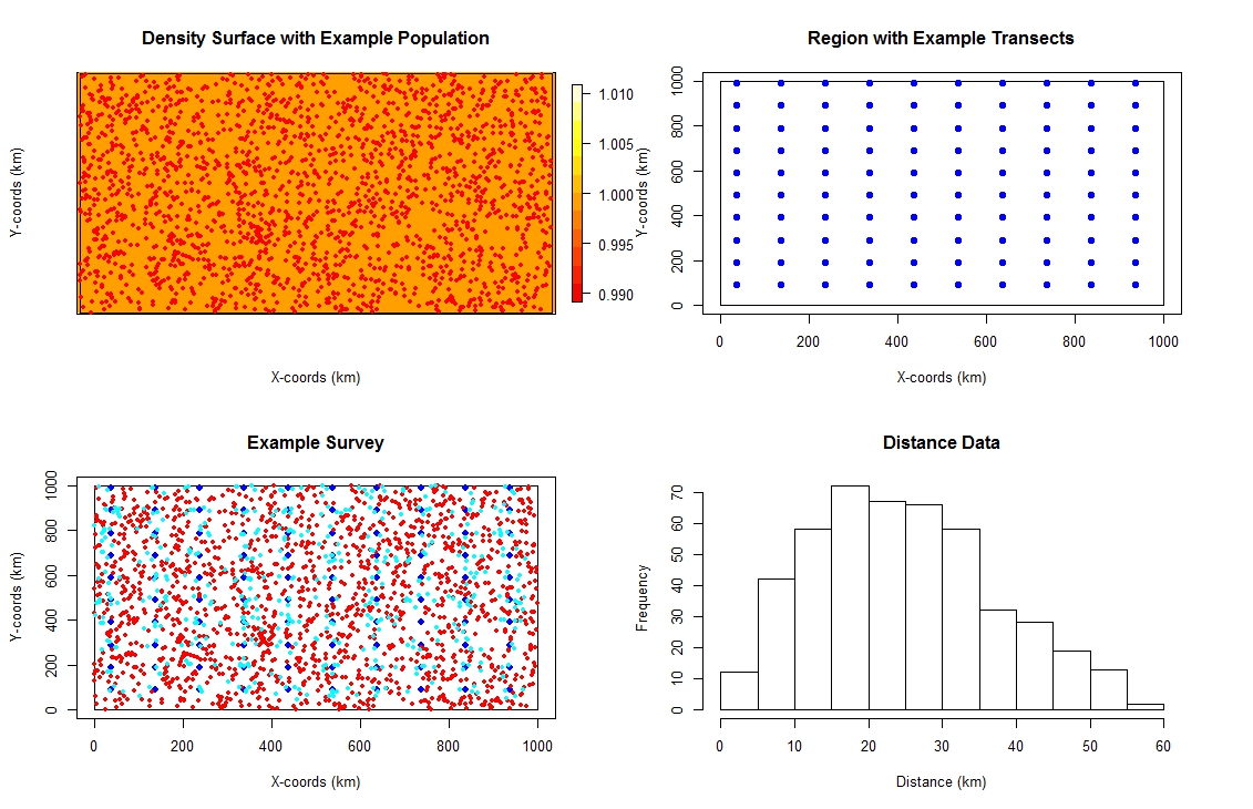
This simulation sets up a square study area of 1000 by 1000 km. The population is a fixed size of 2000 individuals and has an even density throughout the study region. The detectability of the individuals is based on a half-normal detection function with sigma / scale parameter of 20km and sightings are truncated at 60km (a rather optomistic detection function!). The survey design uses a systematic grid of point transect spaced at 100 km intervals. The resulting data are analysed by fitting a half-normal detection function.

#Load DSsim
library(DSsim)

# Create coordinates for a 1000 by 1000 km study region
coords <- list()
coords[[1]] <- list(data.frame(x = c(0, 0 , 1000, 1000, 0), 
                               y = c(0, 1000, 1000, 0, 0))) 

# Create survey region
region <- make.region(coords = coords, units = "km")
plot(region)

# Create flat density surface
density <- make.density(region)
# Plotting density grid as points (the default style)
plot(density)
plot(region, add = TRUE)

# Create a population of 2000, need to give it non default region and density
pop.desc <- make.population.description(region, density, N = 2000)

# Define detectability, by default a half normal (hn) detection function will be used
detect <- make.detectability(scale.param = 20, truncation = 60)

# specify design
# default for point is a systematic placement with a spacing of 100
design <- make.design("point")

# Define analysis
analyses <- make.ddf.analysis.list(dsmodel = list(~cds(key = "hn", formula = ~1)), 
                                   criteria = "AIC",
                                   truncation = 60)

# Put everything together as a simulation
sim <- make.simulation(999, 
                       region.obj = region, 
                       population.description.obj = pop.desc, 
                       detectability.obj = detect, 
                       design.obj = design, 
                       ddf.analyses.list = analyses)

# Let's set a seed to check our results match
set.seed(735)

# Check the setup
check.sim.setup(sim)

# Run the simulation
sim <- run(sim, run.parallel = TRUE, max.cores = 4)

# View the results
summary(sim)

GLOSSARY
--------

Summary of Simulation Output

Region          : the region name.
No. Repetitions : the number of times the simulation was repeated.
No. Failures    : the number of times the simulation failed (too
                  few sightings, model fitting failure etc.)

Summary for Individuals

Summary Statistics:
   mean.Cover.Area : mean covered across simulation.
   mean.Effort     : mean effort across simulation.
   mean.n          : mean number of observed objects across 
                     simulation.
   no.zero.n       : number of surveys in simulation where 
                     nothing was detected.
   mean.ER         : mean encounter rate across simulation.
   mean.se.ER      : mean standard error of the encounter rates 
                     across simulation.
   sd.mean.ER      : standard deviation of the encounter rates 
                     across simulation.

Estimates of Abundance:
   Truth            : true population size, (or mean of true 
                      population sizes across simulation for Poisson N.
   mean.Estimate    : mean estimate of abundance across simulation.
   percent.bias     : the percentage of bias in the estimates.
   RMSE             : root mean squared error/no.successful reps
   CI.coverage.prob : proportion of times the 95% confidence interval 
                      contained the true value.
   mean.se          : the mean standard error of the estimates of 
                      abundance
   sd.of.means      : the standard deviation of the estimates

Estimates of Density:
   Truth            : true average density.
   mean.Estimate    : mean estimate of density across simulation.
   percent.bias     : the percentage of bias in the estimates.
   RMSE             : root mean squared error/no.successful reps
   CI.coverage.prob : proportion of times the 95% confidence interval 
                      contained the true value.
   mean.se          : the mean standard error of the estimates.
   sd.of.means      : the standard deviation of the estimates.

Detection Function Values

 mean.observed.Pa : mean proportion of animals observed in the covered 
                    region.
 mean.estimte.Pa  : mean estimate of the proportion of animals observed 
                    in the covered region.
 sd.estimate.Pa   : standard deviation of the mean estimates of the 
                    proportion of animals observed in the covered region.
 mean.ESW         : mean estimated strip width.
 sd.ESW           : standard deviation of the mean estimated strip widths.
Region:  region
No. Repetitions:  999
No. Failures:  0

Design:  Systematic Point Transect
   design.axis  =  0
   spacing  =  100

Population Detectability Summary:
    key.function  =  hn
    scale.param  =  20
    truncation  =  60

Analysis Summary:
   Candidate Models:
      Model  1 :  ~ cds(key = "hn", formula = ~1)  was selected  999  time(s).
   criteria  =  AIC
   truncation  =  60

Summary for Individuals

Summary Statistics

  mean.Cover.Area mean.Effort   mean.n no.zero.n  mean.ER mean.se.ER sd.mean.ER
1         1130973         100 481.7728         0 4.817728   0.224798  0.2161754


Estimates of Abundance (N)

  Truth mean.Estimate percent.bias   RMSE CI.coverage.prob mean.se sd.of.means
1  2000       1978.28        -1.09 135.26             0.95  134.01      133.57


Estimates of Density (D)

  Truth mean.Estimate percent.bias         RMSE CI.coverage.prob      mean.se  sd.of.means
1 0.002   0.001978284    -1.085784 0.0001352564        0.9469469 0.0001340121 0.0001335687


Detection Function Values

  mean.observed.Pa mean.estimate.Pa sd.estimate.Pa mean.ESW sd.ESW
1             0.22             0.22           0.01    12.95   0.65