Nested Actoustic Point Simulation

This simulation demonstrates a nested point transect design developed to investigate acoustic survey techniques using two different types of detector. Acoustic detectors which can determine distance are very expensive to make and deploy but more simple detectors cannot determine the distance detections were made at.

This simulation implements a design using a combination of these two types of detector. The distances collected from the complex detectors are used to fit the detection function while the encounter rate is obtained from all detectors.

It is important to understand that to replicate reality truncation distances should be very large (where probability of detection is extremely low) as it will not be possible when carrying out the actual surveys to determine which detections on the simple detectors are within a truncation distance and which are not.

# load DSsim
library(DSsim, quietly = TRUE)

# Set seed so reproducible
set.seed(285)

# Create a two strata study area
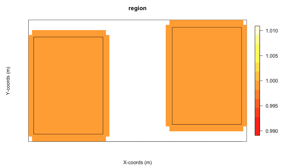
poly1 <- data.frame(x = c(0,0,100,100,0), y = c(0,100,100,0,0))
poly2 <- data.frame(x = c(200,200,300,300,200), y = c(10,110,110,10,10))
coords <- list(list(poly1), list(poly2))
# Make the region with the coordinates
# All other values are left as default implying units are in metres, and strata will 
# be named "A" and "B" and study region named "region".
region <- make.region(coords = coords)
plot(region)

# Create a constant density surface
# The default parameters will mean that the x and y spacing will be 5 and the 
# underlying surface will have a constant value of 1
density <- make.density(region)
# Plot the density surface in block style
plot(density, style = "blocks")
plot(region, add = TRUE)

# Make population with 500 individuals in each strata
pop.desc <- make.population.description(region, 
                                        density, 
                                        N = c(500,500), 
                                        fixed.N = TRUE)

# Make the detectability description
detect <- make.detectability(key.function = "hn", 
                             scale.param = 5, 
                             truncation = 15)

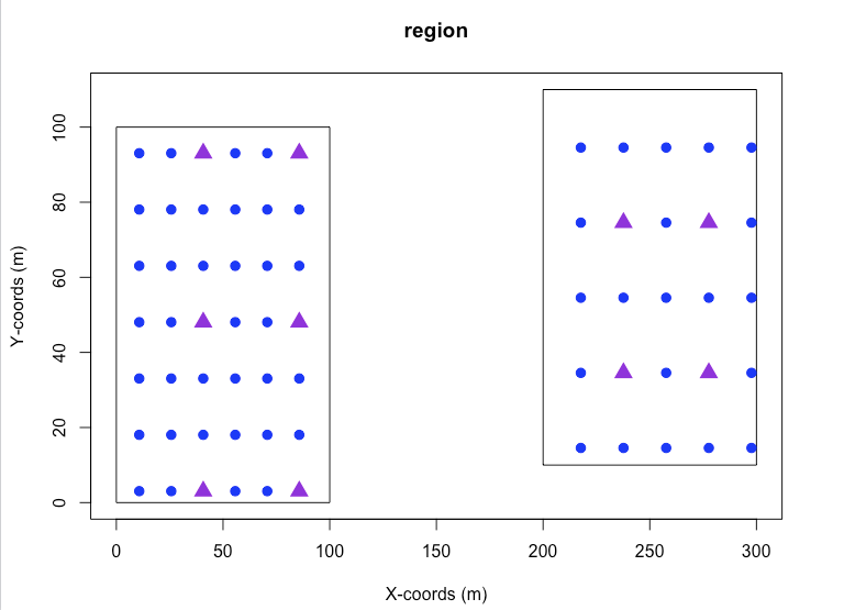
# Define the survey design
# Strata 1 - will have a spacing of 15 and 3 spaces between complex detectors
# Strata 2 - will have a spacing of 20 and 2 spaces between complex detectors
design <- make.design(transect.type = "point", 
                      design.details = "nested", 
                      spacing = c(15,20), 
                      design.axis = c(0, 0), 
                      nested.space = c(3,2))

# Generate some example transects
transects <- generate.transects(design, region = region)
plot(region)
# Purple triangles are complex detectors (record distances)
# Blue circles are simple detector (do not record distances)
plot(transects)

# Define the analyses
analyses <- make.ddf.analysis.list(dsmodel = list(~cds(key = "hn", formula = ~1)), 
                                   method = "ds", 
                                   truncation = 15)

# Create the simulation
point.sim <- make.simulation(reps = 999, 
                             single.transect.set = FALSE, 
                             region.obj = region, 
                             design.obj = design, 
                             population.description.obj = pop.desc, 
                             detectability.obj = detect, 
                             ddf.analyses.list = analyses)

# Check simulation setup
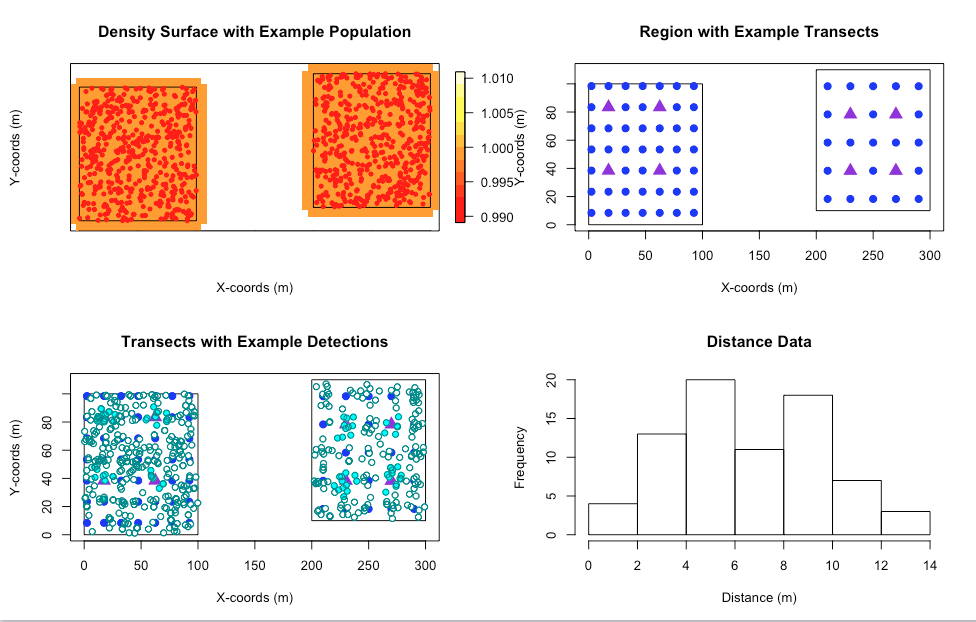
check.sim.setup(point.sim)

In this simulation setup we can see that there are two types of detections in the bottom left plot, those with shaded cyan circles and those with unfilled circles. The shaded circles represent the detections where distances were recorded and the unfilled circles represent the detections where no distance was recorded. We can see that as expected the shaded circles appear in clusters around the complex detectors represented by the purple triangles. The unfilled detections (those without distances) will be associated with the simple detectors indicated by the solid blue circles.

point.sim <- run(point.sim)
summary(point.sim, description.summary = FALSE)

Region:  region
No. Repetitions:  999
No. Failures:  0

Design:  Systematic Nested Point Transect
   nested.space  =  3 2
   design.axis  =  0 0
   spacing  =  15 20

Population Detectability Summary:
    key.function  =  hn
    scale.param  =  5
    truncation  =  15

Analysis Summary:
   Candidate Models:
      Model  1 :  ~ cds(key = "hn", formula = ~1)  was selected  999  time(s).
   criteria  =  AIC
   truncation  =  15

Summary for Individuals

Summary Statistics

      mean.Cover.Area mean.Effort   mean.n mean.n.miss.dist  mean.ER mean.se.ER sd.mean.ER
A            31311.21     44.2963 317.7728         282.9149 7.198031  0.4285971  0.4063250
B            17671.46     25.0000 179.8358         135.0060 7.193433  0.5673445  0.5307190
Total        48982.67     69.2963 497.6086         417.9209 7.190676  0.3428327  0.3238835

Estimates of Abundance (N)

      Truth mean.Estimate percent.bias   RMSE CI.coverage.prob mean.se sd.of.means
A       500        489.98        -2.00  64.05             0.96   67.27       63.29
B       500        490.17        -1.97  72.17             0.95   71.93       71.54
Total  1000        980.15        -1.99 128.67             0.96  130.40      127.19

Estimates of Density (D)

      Truth mean.Estimate percent.bias        RMSE CI.coverage.prob     mean.se sd.of.means
A      0.05    0.04899792    -2.004155 0.006404649         0.958959 0.006727438 0.006328939
B      0.05    0.04901679    -1.966413 0.007217421         0.954955 0.007193382 0.007153719
Total  0.05    0.04900736    -1.985284 0.006433529         0.955956 0.006520073 0.006359673

Detection Function Values

  mean.observed.Pa mean.estimate.Pa sd.estimate.Pa mean.ESW sd.ESW
1             0.04             0.21           0.03     3.16   0.39