In this project, I used what I have learned about deep neural networks and convolutional neural networks to classify 43 traffic signs using the German Traffic Sign Dataset. I trained a model based on LeNet architecture so it can decode traffic signs from the datasets. After the model was trained, I then tested my model performance on the validation dataset to find tune the hyperpromaters. Once the final model is selected, I used the model to test on new images of traffic signs I found on the web.
The steps of this project are the following:
- Load the data set (training, validation, test)
- Explore, summarize and visualize the data set
- Pro-process, design, train and test a model architecture
- Use the model to make predictions on new images
- Analyze the softmax probabilities of the new images
- Summarize the results with a written report
- Jupyter
- NumPy
- SciPy
- scikit-learn
- TensorFlow
- Matplotlib
- OpenCV
The three datasets are pickled data which are providing a dictionary with 4 key/value pairs:
- 'features' is a 4D array containing raw pixel data of the traffic sign images, (num examples, width, height, channels).
- 'labels' is a 1D array containing the label/class id of the traffic sign. The file signnames.csv contains id -> name mappings for each id.
- 'sizes' is a list containing tuples, (width, height) representing the original width and height the image.
- 'coords' is a list containing tuples, (x1, y1, x2, y2) representing coordinates of a bounding box around the sign in the image.
The sizes of the datasets are:
- The size of training set is 34799.
- The size of the validation set is 4410.
- The size of test set is 12630.
- The shape of a traffic sign image is (32, 32, 3), each is a RGB colored image.
- The number of unique classes/labels in the data set is 43.
Noticed that LeNet accepts input of 32 x 32 x C, the dataset is ready to feed in the LeNet with or without grayscale the images.
The image quality are diversified with some of them are fairly good while others are low quality to recognize the type of sign visually.
Training Dataset:
Validation Dataset:

Test Dataset:

The 43 classes in each dataset are distributed fairly in the similar ratio, below shown the statistics:

Generate additional data for training:
With several experimental trainings and validatings for the model performance, I found an overfitting problem that the dropout could not solve well. I plotted the images from both dataset and found out the reason for that was due to the data in the validation dataset are more challenging than the data in the training dataset. As a first step, I decided to augment the training dataset by applying random blurring, brightening, and rotating techniques to add more challenging data to the training set to match closely with the real-road situation. I finally chose to augment 30% images for each traffic sign class from the training dataset, then merged these augmented new images with the training dataset to form an expanded new training dataset. The total number of training data was brought up to 46,892 from 34,799. Here is an example of an original iamge and an augmented image:

As a last step, I then decided to convert the images to grayscale, and normalized them in training, validation, and test datasets. The method for normalization is using Min-Max scaling to a range of [0.0, 1.0].
def normalize_grayscale(image_data):
    a = 0.0
    b = 1.0
    grayscale_min = 0
    grayscale_max = 255
    return a + ( ( (image_data - grayscale_min)*(b - a) )/( grayscale_max - grayscale_min ) )
Here is an example of a traffic sign image before and after grayscaling. Grayscaled and Normalized image
The difference between the original data set and the augmented data set is that the augmented data set contain lower quality of images such as blurrer, brightening light, or from from different angles to a traffic sign. It feeds data with more diverse perspectives to each class labels to produce a more stable model for prediction.
My final model is based on LeNet architecture, with added dropout in the last fully connected layer to prevent overfitting. The LeNet model overview is as follows (noticed the final fully connected OUTPUT layer is 43 rather than 10):

My final model consisted of the following layers:
| Layer | Description |
|---|---|
| Input | 32x32x1 grayscaled image |
| Layer 1 Convolutional 5x5 | 1x1 stride, VALID padding, outputs 28x28x6 |
| RELU | |
| Max pooling | 2x2 stride, VALID padding, outputs 14x14x6 |
| Layer 2 Convolution 5x5 | 1x1 stride, VALID padding, outputs 10x10x16 |
| RELU | |
| Max pooling | 2x2 stride, VALID padding, outputs 5x5x16 |
| Flatten | output 400 |
| Layer 3 Fully connected | input 400, output 120 |
| RELU | |
| Layer 4 Fully Connected | input 120, output 84 |
| RELU | |
| Dropout | keep_probl = 50% |
| Layer 5 Fully Connected | input 84, output 43 |
To train the model, I used tf.train.AdamOptimizer function for training the CNN model. The Adam optimizer is a robust stochastic gradient-based optimization method suited for nonconvex optimization and machine learning problems.
rate = 0.0005
BATCH_SIZE = 128
EPOCHS = 200
logits = LeNet(x)
cross_entropy = tf.nn.softmax_cross_entropy_with_logits(labels=one_hot_y, logits=logits)
loss_operation = tf.reduce_mean(cross_entropy)
optimizer = tf.train.AdamOptimizer(learning_rate = rate)
training_operation = optimizer.minimize(loss_operation)
4. Describe the approach taken for finding a solution and getting the validation set accuracy to be at least 0.93
My final model results were:
- training set accuracy: 0.757
- validation set accuracy: 0.960
- test set accuracy: 0.933
What was the first architecture that was tried and why was it chosen?
I chose the LeNet architecture as its a multilayer Perceptron algorithm working well on the MNIST dataset. I did not use dropout method at first, which resulted a heavy overfitting with a low valadiation accuracy, so I tried to add the dropout in different layer. The current model is to have the dropout before the final fully connected layer which produced a higher validation accuracy (0.960) than the other experiments.
What were some problems with the initial architecture?
The initial architecture produce a higher training accuracy but a much lower validation accuracy (overfitting). I added dropout before the last fully connected layer, meanwhile I took lots of efforts in pre-processing 30% of the images randomly with blurring, rotating, and brightening which are then added into the new training dataset. It turned out it helps with reducing the overfitting problem.
Which parameters were tuned? How were they adjusted and why?
With the newly added augmented images, the training dataset is relatively large. A slower learning rate of 0.0005 learned better than learning rate of 0.001. Although a higher epochs shall produce a better model, I found with current preprocessed data and model architecture, a epochs of 100 is about the highest level the model can learn the most from current data. My current training on 200 epochs (0.960 validation accuracy) helps very little with model improvement comparing with 100 epochs (0.951 validation accuracy).
How does the final model's accuracy on the training, validation and test set provide evidence that the model is working well?
The training accuracy is much lower than the validation accuracy due to the data augmentation that reduced the data quality in the training dataset. I trained 200 EPOCHS with 128 BATCH_SIZE, so the total number of samples images used are 55% of the total samples in the training dataset. The final training accuracy is increased from 0.755 on epoch 50 to 0.757 on epoch 200 with a slower improvement rate, but the validation accuracy rate is increased from 0.947 on epoch 50 to 0.960 on epoch 200.
The final learning rate is set to 0.0005, and with this relatively larger training data, the slower learning rate works better to tune a higher accuracy model.
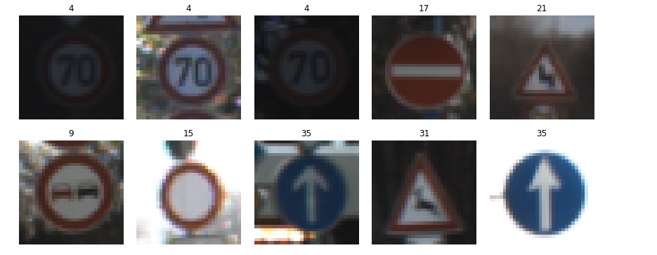
Here are five German traffic signs that I found on the web:

2. Discuss the model's predictions on these new traffic signs and compare the results to predicting on the test set
The model was able to correctly guess 6 of the 8 traffic signs, which gives an accuracy of 75%. This has similar accuracy on newly expanded traing dataset with data augmentation. Validation accuracy and test accuracy are higher, they are respectively 0.960 and 0.933.
3. Describe how certain the model is when predicting on each of the five new images by looking at the softmax probabilities for each prediction. Provide the top 5 softmax probabilities for each image along with the sign type of each probability
The prediction result for the eight new images are:
| Label | Prediction | Probabilities |
|---|---|---|
| Right-of-way at the next intersection | Right-of-way at the next intersection | |
| Priority road | Priority road | |
| Speed limit (60k/h) | Speed limit (60k/h) | |
| Keep right | Keep right | |
| General Caution | General Caution | |
| Speed limit (30k/h) | Speed limit (50k/h) (probability of 0.64) | 2nd guess (probability of 34) predict Speed limit (30k/h)) |
| Turn left ahead | Turn left ahead | |
| Roadwork | Bicyble crossing (probability of 0.62) | 2nd guess (keep left, probability of 0.34), 3rd guess(Bumpy Road, probability of 0.03), |
4th guess (Roadwork, probability of 0.02) |
For the first mis-predicted image, the model is relatively unsure of whether it is a 30k/h speed limit sign or 50k/h speed limit sign. The model gussed with 64% for 50k/h speed limit, and 34% for 30k/h speed limit.
Mis-classification 1: Speed limit (30k/h)

For the second mis-predicted image, the top five soft max probabilities were shown as follows. The images among the correct label and wrongly predicted labels contain pariticial simalities. Such as, pedestrian are shown on both roadwork sign and bicycles corssing signs, which confused the model. Further work can be focusing on improving the model with feeding more on these data to fine tune the model accuracy on these relatively difficult classes.
Mis-classification 2: Roadwork

- Download the German Traffic Sign Dataset. This is a pickled dataset in which we've already resized the images to 32x32.
- Clone the project and start the notebook.
git clone https://github.com/zmandyhe/traffic-sign-classifier
jupyter notebook Traffic_Sign_Classifier.ipynb
Follow the instructions in the Traffic_Sign_Classifier.ipynb notebook.