Registration Trials for THINC Lab Undergraduate research
Sonia Rao under supervision of Dr. Prashant Doshi
Work was presented at UGA CURO 2020 Symposium
relevant 3d point cloud utility scripts that aided this project
code from 3D Smooth Net and scripts
2 sets of matching binary 6D point cloud data with varied # keypoints and 3dSN features and results
python package requirements to use utility functions and 3dSN
SA-Net: Deep Neural Network for Robot Trajectory Recognition from RGB-D Streams
State-Action (SA) detection is a vital step for Learning from Demonstration (LfD), the concept by which a robot is able to mimic a human learner without explicit programming. LfD consists of an initial network trained to recognize all states or actions of any relevant features located within a video, known as SA detection. Another network is created to draw insight about which states and actions correspond, and in which order. The composite process yields a network that is able to recognize behavior patterns which can then be transferred to a robotic agent. In a 2019 study, Sloan et al. developed a novel SA detection network as the first step to a larger LfD pipeline. This network is dubbed SA-Net, and is able to recognize simple SA pairs in a mapped grid environment. Although this model performed with high accuracy, situations with increased SA complexity and a greater number of input modalities poses a novel challenge for SA-Net. In late 2019, the project expanded to include 2 input streams instead of 1. Each stream is captured with a Kinectv2 which is a household RGBD camera originally developed by Microsoft for kinetic video gaming. This work explores different ways to combine these modalities as a pre-cursor to further SA-Net development.
Initial SA-Net environments:

Multimodal fusion is the process by which integration of multiple input modalities yields a more complete input environment. We seek to integrate both kinect streams such that future iterations of SA-Net can capture more information about objects in a given video stream. The largest challenge in integrating kinect streams is that the data streams are not associated on any same plane. That is, Kinect A's (x,y,z) depth field does not correspond to Kinect B's (x,y,z) depth field. Hence, without multi-modal fusion, the network would have no way to determine whether the kinects are seeing the same object or two different and identical objects. Although fusion research has grown fairly recently with the rise of deep networks, there are three commonly used techniques for multimodal fusion: early fusion, late fusion, and hybrid fusion. Early fusion is the process where multiple streams are combined into one cohesive input prior to any feature learning. Late Fusion is the process by which a network learns features of each input stream separately and independently, and later combines input stream features through matrix operations. Hybrid fusion is a combination of the two where input streams are partly combined prior to feature learning, and further refined after feature learning. After examining all three methods, we decided upon early fusion in the interest of modularity between input processing and network development.
Below is an example of multi-stream fusion. Although each segment represents a different viewpoint, each viewpoint can be combined to contain a more complete view of the scene.


THINC Lab is developing a novel LfD pipeline in which a robot will be able to perform a pick and place task. Given a conveyor belt scattered with onion of varying quality, the robot will be able to decide the quality of each onion based on visual inspection, and then sort the onions into two bins for 'Good onions' and 'Bad onions' respectively.


Prior to early-fusion trials, I needed to collect two streams of kinect data with each stream adequately capturing a large amount of complex states and actions for the task at hand. Using the Robot Operating System (ROS) module for kinectv2, me and my colleague Farah collected over 50 GB of data to find the optimal kinect locations. We placed one kinect where all motions of the expert, relevant scene objects, and actions could be clearly scene. This included: directly in front of the expert and conveyor, to either side of the expert, and angled above the expert. The second kinect necessarily had to capture the expert's viewpoint. This is because the pipeine will eventually learn to make decisions that mimic the expert. If the expert sees a blemish upon closer inspection of an object, and thus places it in the proper bin, the model will need to know what visual trigger caused the expert to take this action. As such, we experimented with camera angles behind and above the expert so that the expert's hand holding the onion is visible with as much conveyor belt shown as possible.
Examples of data collected:


The data were in .bag file format as per ROS requirements. Each frame is in point_cloud format and has an RGB image component and an XYZ depth component. I remain unsure whether the synchronization process would be more seamless with different hardware, but we worked with roughly time-space-kinect synchronized data for the project duration.
Because of our workspace constraints, we only had the bandwidth to connect each kinect to a single computer, rather than connecting both kinects to one computer. We first tried to connect the computers over the network such that we could start both streams at the same time. Howeverm this resulted in vastly different amounts of data recorded, as our computer could not handle the influx of data. When we started it from different computers, a smaller time lag persisted. The streams would begin at different times, have slightly different frame timestamps, and most bizzarely would have inconsistencies between the depth and RGB frame timestamps. That is, for each RGB-D frame in either kinect, the depth component was recorded at 0.75x the speed of RGB component, likely because point cloud data is more resource intensive. To mitigate this, we had to make sure the hardware was being commanded properly. We ensured that the frame rate was at its maximum so that the number of images and number of depth frames recorded were close to similar with minimal lag. Because less depth data ends up being recording, due to hardware and operating system limitations, we limit our dataset to depth frames and their corresponding image frames, and disregard all image frames that do not have a depth frame counterpart. We matched the frames using a time synchronizing utility. As a rough approximation, a 1 minute RGB-D video recorded on both streams would yield about 20-30 image-depth pairs on EACH kinect that were adequately time and scene synchronized.
To capture critical states, actions, and objects, our data collection must abide by the following:
- all onions on the conveyor belt must be visible by one, both, or a combination of the two streams
- the quality of all onions on the conveyor belt must be determinable by one, both, or a combination of the two streams
- all ranges of the expert's hand must be visible by both streams
- one stream must capture the expert's viewpoint when examining individual onions (hand raised to face)
- the bins or bin region must be visible by one, both, or a combination of the two streams
To address the onion on the conveyor, we place one kinect anywhere between directly in front of the observer to 90 degrees either direction. To address the expert's viewpoint, we place the second camera at varying heights above the expert's left or right shoulder. Below is an example of the shoulder camera's perspective with the image and depth frames overlaid; the camera can see much of the conveyor belt and can also detect possible blemishes when the expert investigates an individual onion closer to their face.

close-up of blemish:

Unfortunately, the workspace we were in posed several physical limitations to data gathering. Primarily, there exists a large pole at the center of the room that obstructs direct view of the conveyor belt. You can see the white space in the above examples is part of the pole, and is highly obstructive. It is possible that the locations we chose will not be optimal for other workspaces.
The general idea of ICP is to match corresponding sets of points without knowing the grount truth data association parameters. Because it is generally impossible to determine the optimal relative rotation/translation in one step if the correct correspondences are not known, the algorithm iteratively computes closest points and thresholds. The algorithm is as follows: generate/determine corresponding points, compute rotation and translation via singular value decomposition, apply those matrices on set to be registered, compute error. If error decreases, repeat steps with updated values for rotation and translation computation. While this method has been around for a while, it is challenging on such a large set of points without explicit mapping. This is known as local registration, whereas global registration methods such as RANSAC are generally more sophisticated. To use RANSAC, or RANdom SAmple Consensus, random points are picked from the source point cloud. Their corresponding points in the target point cloud are detected by querying the nearest neighbor in the 33-dimensional FPFH feature space. A pruning step takes fast pruning algorithms to quickly reject false matches early. We used open3d's implementation of ICP and RANSAC, and find that neither method is efficient or high accuracy.
Because ICP and RANSAC did not produce very satisfactory results, we moved onto exploring novel deep learning methods. The advantage of deep learning based methods over traditional methods is that, usually, deep networks are able to leverage high dimensional features which can then be used for matching. There are several existing deep networks that convert RGB-D data into high dimensional features which can then be used with matching algorithms such as RANSAC. The primary obstacle to using these methods is that our data is not only unmatched, but both streams are on different coordinate planes. Thus, we need a deep learning algorithm that is able to firstly convert RGB-D data into high-dimensional features, and secondly register those features on the same coordinate system. From there, we can use those features as inputs to RANSAC for a more cohesive early-fused input to the revised SA-Net.
The Perfect Match: 3D Point Cloud Matching with Smoothed Densities In late 2019, I came across this paper by researchers at ETH Zurich who were working on a similar issue: tackling data registration and RGB-D feature learning simultaneously. Check out the 2019 CVPR paper in the above link for details on their novel method known as 3dSmoothNet. For the remainder of the project, my registration trials revolved around adapting and optimizing 3DSmoothNet for our data.
Due to limited access to a GPU server, I set up 3DSmoothNet on a Google Cloud Platform compute engine instance with Nvidia P100 GPU and 4 CPU cores. Every new user gets a large amount of free GPU credits which was sufficient for the project until I gained access to a regular GPU server. If you don't have GPU access, I recommend GCP.
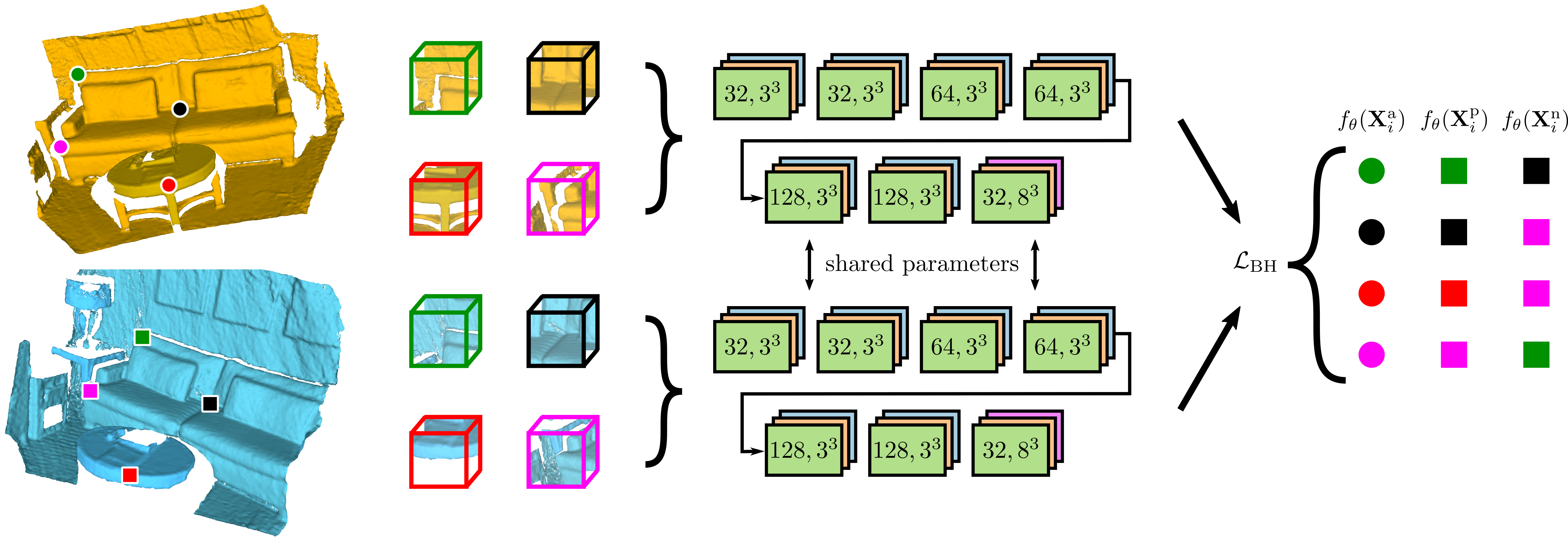
The general idea of 3DSmoothNet is matching point clouds via fully convolutional layers and voxelized smoothed density value (SDV) representations. SDV grids are computed per interest point and aligned to a local reference frame (LRF) to achieve rotation invariance. This allows their approach to be sensor agnostic. The 3D point cloud descriptor achieves high accuracy on 3DMatch benchmark data set, outperforming the SOTA with only 32 output dimensions. This very low output dimension allows for near realtime correspondence. 3DSmoothNet trained only on RGB-D indoor scenes achieves 79.0% average recall on laser scans of outdoor vegetation, suggesting that 3dSN's model generalizes well to a wide variety of scenes. Because of this, I thought that 3dSN might be a good fit for our indoor workspace setting, and real-time registration preference. Ideally one pass through 3dSN will be sufficient to produce a translation matrix that would generalize to all frames in a video, but if that isn't the case, this method would be able to produce fast results per set.
below is a diagram of the 3dSN architecture. For training, the keypoints necessarily need to correspond with a known mapping.
Our process to use 3dSN pre-trained model:
- Collect two streams of RGB-D data that contain varying levels of commonality (anywhere from 20%-80%)
- Unpack .bag files using ROS
- Extract time-synchronized data between the two streams (at least 1 pair)
- Convert point cloud entities into binary point-clouds (default is ASCII)
- Generate Index files of Key points (see below section)
- Parametrize using 3dSN SDV
- Perform inference via 3dSN pre-trained model
- Match using RANSAC on high-dim features
- Obtain translation matrix
Our process to train on top of their pre-trained model:
- Collect and process data (same as above)
- Extract at least 30 pairs of time-synchronized pairs across a wide variety of expert motion
- Manually select key points (see below)
- Generate index files with keypoints and nearest neighbors
- Parametrize keypoints using 3DSN SDV
- Create mapping of keypoints using rough translation matrix
- Convert mapped parametrized inputs into .tfrecord format
- Train on top of 3dSN weights
- Match using RANSAC on inferred high-dim features
- Obtain refined translation matrix
We will go into more detail below and in utils.
We first explored generating key points from common sections within points. It was unclear from the 3DSN paper what percentage of either point cloud should correspond, and as such we tried varying levels of keypoints, common regions, and data. I found that having around 80% of common regions between the point clouds yielded optimal keypoints. Our process was as such:
- Collect data with 80% common region
- Overlay point clouds and extract common region from each
- Crop common region of point clouds into two new separate clouds
- Generate N random points from each cloud
- Feed into 3dSN
Because in this case we are only testing using 3dSN's pre-trained model, we are able to use randomly generated keypoints without any mapping function. 3dSN coupled with RANSAC is able to infer the rough correspondances of keypoints without explicit direction. While that's convenient, this method did not perform super well due to scalability issues.
Our individual point clouds contain over 1 million points. The cropped common region, with 80% similarity, contains anywhere from 500,000 points to 750,000 points. To randomly generate keypoints that have rough correspondences, we would need to generate a vast number of keypoints, likely over 50,000. It is impossible to parametrize and infer even a fraction of that. I tried repeating the process with downsampled clouds, but found that the results suffered.
Because the keypoints are no longer selected randomly, there is no need to have a vast number of keypoints or an extensive common region. However, I find that having 60% common region was still preferred for our workspace settings. Because our workspace was small, having greater than 40% different regions usually meant that our kinects were angled significantly differently. It is challenging to infer correspondences between matching points if they are visually different. Our process was as follows:
- collect data with >60% common region
- Use the point picker utility in utils to select key points, quantity of nearest neighbors
- Repeat for second cloud
- Turn points into index file
- feed into 3dSN
I experimented with over 15 levels of nearest neighbors ranging from 2 to 5,000. I find that there's a computational bottleneck with using over 500 nearest neighbors. Additionally with too many keypoints, the RANSAC matching performed poorly since several of the features showed the same points. Usually 50 to 200 nearest neighbors and ~20 keypoints per cloud are sufficient for parametrization and inference.
Below images show chosen keypoints. Each keypoint was present in both clouds without much visual difference. Additionally, the sphere around each point can be thought of as a "neighborhood" of nearest neighbor points that are using in the testing pipeline.


Testing results using this method were satisactory. The planes visually look very aligned, and important objects (e.g. blemished onion) that were obscured in either cloud seem to be cohesively fused. However, it was still possible for us to obtain better results by training the model using our data.
To update the 3dSN for our data, I needed to collect data and transfer it to .tfrecord format. After corresponding with the authors, I realized that to do so, I need to first generate keypoints for both clouds and second create an explicit mapping of each keypoint to its corresponding match in the other point cloud. The authors of 3dSN used the publically available 3dMatch dataset to develop their model and train their weights. This data has over 10,000 pairs of point cloud data and their corresponding ground truth. This poses a unique challenge. I do not have ground truth data, it would be impossible for us to collect ground truth data, and it would take a long time to collect, process, and generate keypoints for enough data to make a sizable difference to the pre-trained model. As such, I used a matrix refinement method to tune the pre-trained model, rather than shape it entirely to our data.
I started by generating 20 keypoints with 120 nearest neighbors for around 15 corresponding pairs of point clouds. I fed it into 3dSN without modification and obtained a rough translation matrix. The rough matrix can essentially be used to generate mapping of one point cloud to the other. Using the original 20 keypoints with ZERO nearest neighbors, I used the keypoint matching utility to overlay the clouds on the same plane and determine matching points. I then parametrized the points using 3dSN, converted the features into tfrecord using the mapping, and fed it into 3dSN for training.
I find that training with 20 to 50 keypoints did not significantly alter the visual results, and that using the pre-trained 32-dimensional model is generally sufficient for this task.
Without ground truth, it's difficult to visually determine the registration accuracy. The data folder includes a .ply file with the most recent registration trial on the same plane. Unfortunately, the onset of COVID shelter-in-place measures stopped me from collecting new data, which I assumed would be part of the project. I began training trials with about 20 pairs of matched data to explore processing techniques. I assumed that I would be able to collect and process more data for training once I had a better idea of what training and evaluation would entail. As such, I never collected more data and it is possible that training on more data would significantly improve results.
Future work includes:
- Collecting more data showing different state-action pairs
- Using another set of data to test trained model
- Creating a driver program to automatically time-synchronize data from RGB-D video, register data into one plane, and create a new RGB-D video
- Test 3d Object detection methods on registered RGB-D set
- link for public .bag files
Sonia Rao [email protected]
Dr. Prashant Doshi [email protected]
THINC Lab: http://thinc.cs.uga.edu/