ft_linear_regression

42 school project ft_linear_regression could be seen as an entrypoint to the data science branch of 42-school, in the outer-circle holygraph. This project is an introduction the field and does not have the pretention to be a fancy data science project. Machine learning modules, and any module doing the job, are forbidden.

Preview
Subject
- Dataset
- Mandatory
- Bonus
My solution to linear regression
- Usage : venv and run
- Classes and files
- Training : predicting output values with gradient descent algorithm
ft_linear_regression functionalities

Preview

Figure 1. Loss surface visualization. Cost function $J(\theta_0, \theta_1)$ is represented on a log scale.

Figure 2. Model Training. Left panel: normalized dataset scatterplot representation, with the line to the predicted value after training. Right panels: Cost function, $\theta_0$, and $\theta_1)$ are represented through epochs (training iterations).

Subject

The objective is to implement a simple linear regression with a single feature, from scratch. The choice of programming language is free, but should suitable for visualizing data. Using librairies is authorized, except for the ones that does all the work. For example, using python’s numpy.polynomial() function or scikit-learn library would be considered as cheating.

Dataset to train

Monovariate : Car mileage as inputs, car price as output

km	price
240000	3650
139800	3800
150500	4400
...	...

data.csv

Mandatory Part

A first program predict.py is predicting the price of a car for a given mileage. The prediction is based on the following model hypothesis :

estimatePrice(mileage) = θ0 + (θ1 ∗ mileage)

Parameters thetas are set to 0 by default, if training did not occur yet.

A second program training.py is training the model, from a data.csv train set. According to the hypothesis, both parameters thetas are updated with gradient-descent algorithm.

The two programs cannot directly communicate. Model parameters issued from training dataset, should be stored and be accessible independently of runtime (Data persistency).

Bonus part

• Plotting the data into a graph to see repartition.

• Plotting the line resulting from linear regression training into the same graph.

• Calculating the precision of the implemented algorithm.

• Any feature that is making sense

My solution to ft_linear_regression

To implement linear regression from scratch, I chose Python language. Librairies : The power of numpy, a pinch of pandas and matplotlib for visualisation.

Usage

Virtual environment

a virtual environment is necessary so that python and its dependencies are running in an isolated manner, independently from the "system" Python (the host machine).Virtualization with the help of Docker could be a way to do that in a more complex context. Here, only python installer pip, python3 and few libraries are needed.Thus, virtualenv is the most straightforward tool (virtualenv doc. and python doccs), and can install a virtual environment from these shell command :

virtualenv ./venv/
/venv/bin/pip install -r requirements.txt

Makefile capabilities were usedto set up virtual environment for Python, run programs or clean files. Of course, there is no compilation occuring since Python is an interpreted language.

make command will install the virtual environment with dependencies specified in the requirements.txt file.

make predict to execute the predict.py program.

make training to execute the training.py program.

make flake to check for norm with flake8.

make clean to remove __pycache__ and .pyc files.

make fclean to remove the virtual environement after applying the clean rule.

Run

Run with predict.py or training.py

After, that virtual environment and requirements are installed.

Run with virtual environment python

venv/bin/python predict.py

Otherwise Activate of the virtual environment

source /venv/bin/activate

This will change the shell prompt, to (venv) and allow to directly use venv/bin/*. Type only pip or python of the venv with only one word, no need for /venv/bin/ prefix.

python predict.py

Classes and files

graph TD;
  A[predict.py]-->|instanciate|B[class <br> PredictPriceFromModel];
  C{model  <br>  parameters  <br> persistency}--read-->A[predict.py];
  D[training.py]--instanciates-->E[class  <br> CarPriceDatasetAnalysis];
  E[class  <br> CarPriceDatasetAnalysis]-->F[class  <br> LinearRegressionGradientDescent];
  E[class  <br> CarPriceDatasetAnalysis]--writes-->C{model  <br>  parameters  <br> persistency};
  G{car price <br>  training  <br> dataset}--read-->E[class  <br> CarPriceDatasetAnalysis];

Training

Linear regression

The objective is to find a solution to the linear hypothesis model.

For multiple linear regression, the output response ($Y$) linearily depends on a discrete number of $k$ independent variables ($X_j$) also called predictors. With $\theta_j$, as Weights of the hypothesis for $j$ being the feature index number (from 1 to k).

Predicted output $$y = \theta_0 + \theta_1 * x_1 + \theta_2 * x_2 + ... + \theta_k * x_k$$

In our model, the hypothesis is that price is depending only on mileage, therefore $\theta_0$ and $\theta_1$ are the two weigths to be found by our algorithm.

For any x input value, and more specifically any $x_i$, an output predicted value $h(x_i)$ can be calculated with the following linear relationship.

Output predicted value $$h(x_i)=\theta_0 + \Theta_1 * x_i$$

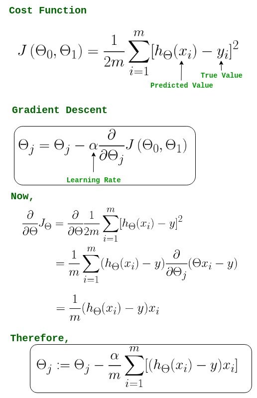
For any given $x_i$, the calculated predicted value $h(x_i)$ might differ from the real value of $y_i$. These residual are specific to each $x_i$ but also to each $[\theta_0, \theta_1]$ pair at any step of learning.

Gradient descent

The linear-fit relationship to the given dataset is based on the Sum of Squared Residuals Method, trying to find the minimize $$\sum_{i=1}^m (h(x_i) - y_i)^2$$ during the learning process,

The cost function of the linear regression $J(\theta_0, \theta_2)$, measures the Root Mean Squared error between the predicted value (pred) and true value (y).

cost function $$J(\theta_0, \theta_1) = \frac{1}{2m} \sum_{k=1}^m (h(x_i)-y_i)^2$$

To implement the gradient descent algorithm, to keeping it simple, the slope of the cost function according to each $\theta$ direction, orientates us toward the minimal cost and tells if that $\theta$ needs to be increased or decreased. In addition to that, it also allows to update the value of that same given $\theta$.

Partial derivative of $J(\theta_0, \theta_1)$ to $\theta_0$ $$\delta(J(\theta_0, \theta_1))/\delta\theta_0 = \frac{\alpha}{m} \sum_{k=1}^m (h(x_i)-y_i)$$

Partial derivative of $J(\theta_0, \theta_1)$ to $\theta_1$ $$\delta(J(\theta_0, \theta_1))/\delta\theta_1 = \frac{\alpha}{m} \sum_{k=1}^m (h(x_i)-y_i)x_i$$

$\alpha$ : Learning Rate of Gradient Descent.

$[\theta_0, \theta_1]$ pair is updated by decrementing $\alpha * partial derivative$ amount. Linear algebra and numpy simplifies the equation translation into python coding language :

partial_derivative = np.zeros(2)
partial_derivative[0] = np.mean(residual)
partial_derivative[1] = np.mean(np.multiply(self.x, residual))
self.theta -= self.alpha * partial_derivative

Developped explanation are found here : geeksforgeeks.com : gradient descent in linear regression articles

In summary

**Basically, at any step of the learning process: The pair $[\theta_0, \theta_1]$ allows to calculate • the cost function J(\theta_0, \theta_2)$ given all the $x_i$ of the trainset. • the partial derivative for $theta_0$ • the partial derivative for $theta_1$ • update the $[\theta_0, \theta_1]$ pair accordingly.