CPS_continuous_plant

CPS Component: Continuous-time Plant (Mobile Robot)

In this example a unicycle type mobile robot is simulated using the hybrid system toolbox. It is assumed that the forward velocity can be either 1 or 0, and the control command is $u\in\mathbf{R}$ . The control input is assumed be remain between $\pm 1$ , i.e., $u \in [U_{\min},\ U_{\max}] := [-1,+1]$ . Moreover, the unicycle is initialized at the origin and required to reach the boundry of a circle of radius $X_{\max}$

Contents

• Mathematical Model
• Simulink Model
• Example Output

The files for this example are found in the package hybrid.examples.mobile_robot :

• initialize.m
• mobile_robot.slx
• postprocess.m

The contents of this package are located in Examples\+hybrid\+examples\mobile_robot (clicking this link changes your working directory).

Mathematical Model

A unicycle mobile robot is a continuous-time nonlinear system. Let $x_1$ and $x_2$ be the position of the unicycle on 2D plane and $x_3$ be the orientation. The kinematics model is given by

$$\begin{array}{ll} \dot x_1 = v \sin x_3\\\ \dot x_2 = v \cos x_3\\\ \dot x_3 = u, \end{array}$$

where the forward velocity $v$ is assumed to be constant, and without loss of generality $v = 1$ . The states and input of the system are $(x_1,x_2,x_3)\in\mathbf{R}^{3}$ and $u \in \mathbf{R}$ , respectively. We express this system as a hybrid control system with the following data:

$$\begin{array}{ll} f(x,u):=\left[\begin{array}{c} \sin x_{3} \\\ \cos x_{3} \\\ u \end{array}\right], & C := \{ (x,u) \in \mathbf{R}^{3} \times \mathbf{R} \mid u \in [U_{\min},\ U_{\max}], x_1^2 + x_2^2 \leq X^2_{\max}\} \\ \\\ g(x,u):=\left[ \begin{array}{c} 0 \\\ 0 \\\ 0 \end{array}\right], & D: = \emptyset \end{array}$$

Simulink Model

The following diagram shows the Simulink model for this example. The mobile robot is represented by the Continuous-time Plant block.

A Continuous-time Plant block contains user-defined a flow map $f$ block and flow set $C$ block.

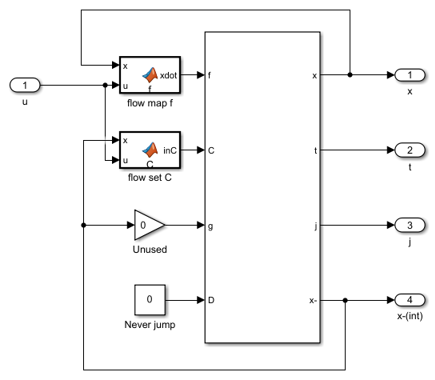
The flow map and flow set functions in this example are included below.

flow map f block

function xdot = f(x, u)
    % Flow map for plant.
    xdot = [sin(x(3)); cos(x(3)); u];
end

flow set C block

function inC  = C(x, u, parameters) 
    % Flow set indicator function for plant.
    x1 = x(1);
    x2 = x(2);
    minU = parameters.minU;
    maxU = parameters.maxU;
    maxX = parameters.maxX;
    if u >= minU && u <= maxU && x1^2+x2^2 <= maxX^2
        inC = 1; % report flow
    else
        inC = 0; % do not report flow
    end
end

The jump set C block is given as a constant block with value zero and the jump map D block is unused.

Example Output

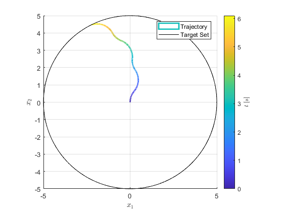
The following plot shows a solution to the closed-loop system. The robot starts at the origin and then drives until it eventually hits the target set, which is a circle with radius 5 centered at the origin.