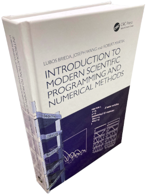
We begin by introducing the concept of numerical integration by developing an algorithm for calculating the trajectory of a tennis ball. The algorithm is first evaluated using "pen and paper". It is then adapted into a spreadsheet, before finally being ported to Python. This example also allows us to introduce basic programming concepts such as functions, variables, as well as random number generators. Here we also compare around a dozen of frequently encountered programming languages.
Chapter 2 introduces Taylor Series and the Finite Difference Method. This method is used to discretize the 2D steady-state heat diffusion equation. Direct and iterative matrixes solvers are introduced. The solver is developed in Python.
This chapter covers various numerical analysis topics such as data filtering, interpolation, quadrature, Newton-Raphson linearization, distribution function sampling, and multigrid solvers.
Chapter 4 is a crash course on C++. C++ is a language commonly found in high-performance codes and software libraries and hence it is imperative to become familiar with concepts such as references, polymorphism, operator overloading, and template arguments. A C++ version of the heat equation solver from Chapter 2 is developed. Results are visualized using Paraview.
Chapter 5 introduces particle methods. Although we describe these methods in the context of gas dynamics, topics covered here are applicable to other disciplines as well. We develop a sample code for free molecular, then collisional, and finally plasma flow around an infinitely long cylinder. The chapter covers mesh-to-particle interpolation, and the computation of macroscopic flow properties such as density, velocity, and temperature from particle data.
This chapter cover mesh-based Eulerian approaches. It discusses stability analysis in the context of several model equations including advection-diffusion, wave, Burger's, and Maxwell's equations. An unsteady version of the heat equation solver is developed. Fluid modeling is demonstrated with the streamfunction-vorticity method. A Vlasov solver for the Boltzmann equation governing evolution of velocity distribution function is also included.
Chapter 7 changes gears and covers development of HTML and Javascript codes that run in a web browser. Such codes not only offer interactivity not easily incorporated into C++ codes, but also allow one to develop programs on lab machines that otherwise may lack a programming environment. We describe rendering using the CPU-based 2D context as well as the GPU accelerated webgl interface.
Chapter 8 covers various topics related to software engineering, including debugging, use of test suites, version control, build systems, libraries, documentation, and coding practices. The LaTeX document setting environment is also discussed.
Chapter 9 introduces parallel programming. It starts by covering profiling for identifying code parts most applicable to parallelization. Multithreading is then introduced. Here we cover the race condition and the use of mutexes for serialization of sensitive code sections. Next, domain decomposition with MPI is discussed. Here we cover deadlock, as well as the use of ghost cells for data transfer. The chapter closes with an overview of graphics card (GPU) processing using CUDA, as well as the use of OpenGL for rendering.
Chapter 10 starts by introducing approaches such as gradient descent and genetic algorithms for finding input parameters for improving agreement with expected results. Machine learning is then introduced and a small dense neural network is constructed for classifying real values. The back propagation method is used to find the optimal neural net weights and biases.
Finally, Chapter 11 covers development of codes running on microcontrollers and FPGAs. Such devices allow for the so-called edge computing in which data analysis is done close to the source of data. We see how to integrate an Arduino microcontroller with a 3rd party sensor. We then cover FPGA programming using the Intel Cyclone development kit and also learn how to utilize Arduino microcontroller that comes with a built-in FPGA.
These examples are meant to be used along with the textbook. Some examples are standalone ``snippets'' used to demonstrate a particular functionality. Such examples can be compiled and executed using
$ g++ file_name.cpp
$ ./a.out
or, if you prefer specifying the output file name and including optimization
$ g++ -O2 file_name.cpp -o app_name
$ ./app_name
Python snippets can be run using
$ python file_name.py
Other examples, such as the various gas dynamics examples in Chapter 5, consist of multiple source files that need to be compiled together as in
$ g++ -O2 *.cpp -o sphere
Simulation results are usually stored in a subfolder results which needs to be created manually before the code is run for
the first time. The reason for this is that prior to C++17, there was no platform-independent way to create directories
in C++. C++17 was not yet universally supported at the time of book writing. Hence to run the code the first time, use
$ mkdir results
$ ./sphere
It is quite likely there are various bugs in the code. Please use the Issues Tracker to identify them so they can be corrected in a future book revision.
Dr. Lubos Brieda: [email protected]