riskmodels: a library for univariate and bivariate extreme value analysis (and applications to energy procurement)

This library focuses on extreme value models for risk analysis in one and two dimensions. MLE-based and Bayesian generalised Pareto tail models are available for one-dimensional data, while for two-dimensional data, logistic and Gaussian (MLE-based) extremal dependence models are also available. Logistic models are appropriate for data whose extremal occurrences are strongly associated, while a Gaussian model offer an asymptotically independent, but still parametric, copula.

The powersys submodule offers utilities for applications in energy procurement, with functionality to model available conventional generation (ACG) as well as to calculate loss of load expectation (LOLE) and expected energy unserved (EEU) indices on a wide set of models; efficient parallel time series based simulation for univariate and bivariate power surpluses is also available.

Requirements

Python >= 3.7

Installation

pip install riskmodels

API docs

https://nestorsag.github.io/riskmodels/

Quickstart

Univariate extreme value modelling

Empirical distributions are the base on which the package operates, and the Empirical classes in both univariate and bivariate modules provide the main entrypoints.

import riskmodels.univariate as univar
import riskmodels.bivariate as bivar

# prepare data
gb_nd, dk_nd = np.array(df["net_demand_gb"]), np.array(df["net_demand_dk"])
# Initialise Empirical distribution objects. Round observations to nearest MW
# this will come n handy for energy procurement modelling, and does not affect fitted tail models
gb_nd_dist, dk_nd_dist = (univar.Empirical.from_data(gb_nd).to_integer(), 
  univar.Empirical.from_data(dk_nd).to_integer())

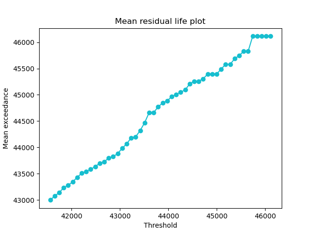
#look at mean residual life to decide whether threshold values are appropriate
q_th = 0.95
gb_nd_dist.plot_mean_residual_life(threshold = gb_nd_dist.ppf(q_th));plt.show()
dk_nd_dist.plot_mean_residual_life(threshold = dk_nd_dist.ppf(q_th));plt.show()

Mean residual life plot for GB at 95%

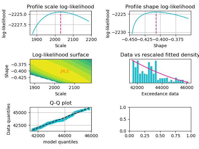
Once we confirm the threshold is appropriate, univariate generalised Pareto models can be fitted using fit_tail_model, and fit diagnostics can be displayed afterwards.

# Fit univariate models for both areas and plot diagnostics
gb_dist_ev = gb_nd_dist.fit_tail_model(threshold=gb_nd_dist.ppf(q_th))
gb_dist_ev.plot_diagnostics();plt.show()
dk_dist_ev = dk_nd_dist.fit_tail_model(threshold=dk_nd_dist.ppf(q_th))
dk_dist_ev.plot_diagnostics();plt.show()

The result is a semi-parametric model with an empirical distribution below the threshold and a generalised Pareto model above. Generated diagnostics for GB's tail models are shown below.

Diagnostic plots for GB model

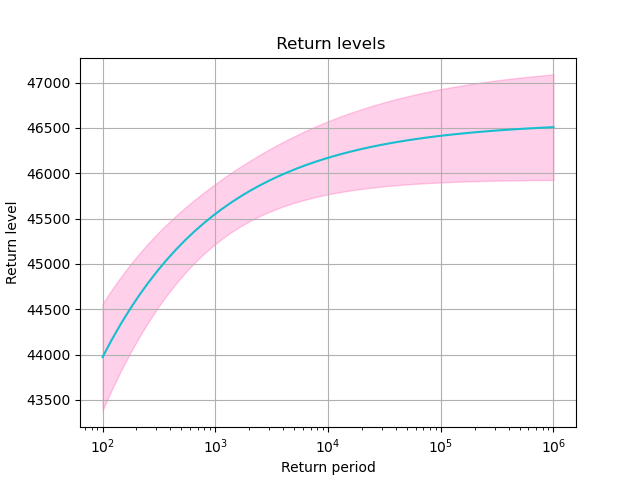
Return levels for GB

Bivariate extreme value modelling

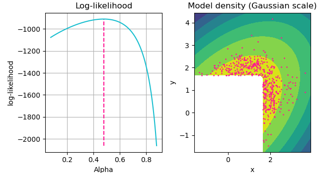
Bivariate EV models are built analogously to univariate models. When fitting a bivarate tail model there is a choice between assuming "strong" or "weak" association between extreme co-occurrences across components ¹. The package implements a Bayesian factor test, shown below, to help justify this decision. In addition, marginal distributions can be passed to be used for quantile estimation in the fitting procedure.

Data sample scatterplot (x-axis: GB, y-axis: DK)

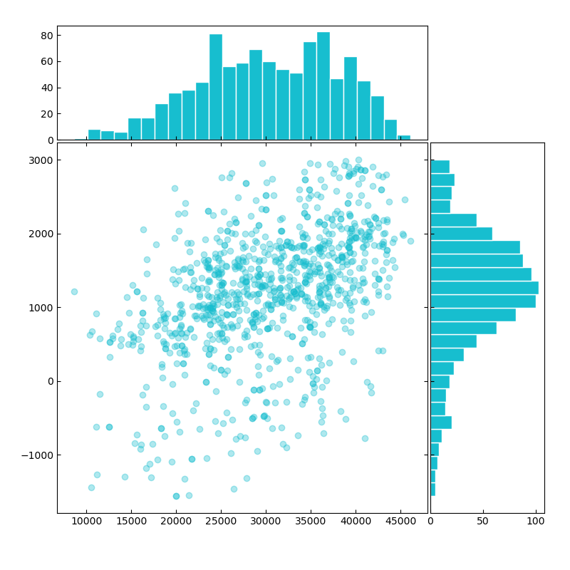
# set random seed
np.random.seed(1)
# instantiate bivariate empirical object with net demand from both areas
bivar_empirical = bivar.Empirical.from_data(np.stack([gb_nd, dk_nd], axis=1))
bivar_empirical.plot();plt.show()

# test for asymptotic dependence and fit corresponding model
r = bivar_empirical.test_asymptotic_dependence(q_th)
if r > 1: # r > 1 suggests strong association between extremes
  model = "logistic"
else: # r <= 1 suggests weak association between extremes
  model = "gaussian"

bivar_ev_model = bivar_empirical.fit_tail_model(
  model = model,
  quantile_threshold = q_th,
  margin1 = gb_dist_ev,
  margin2 = dk_dist_ev)

bivar_ev_model.plot_diagnostics();plt.show()

Bivariate model's diagnostics plots