Pyoelectricity

This repository contains the code behind our publication

Annihilation of action potentials induces electrical coupling between neurons

Please cite as:

Schlötter Moritz, Maret Georg, Kleineidam Christoph J (2023) Annihilation of action potentials induces electrical coupling between neurons eLife 12:RP88335 doi.org/10.7554/eLife.88335

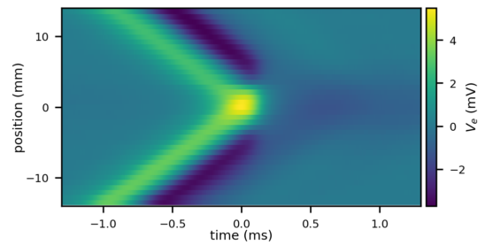
We analyze colliding Action Potentials (APs) in detail to test and refine models of excitable membranes. The results validate the Tasaki-Matsumoto (TM) model and confirm its behavior upon collision. The TM model predicts the extracellular current generated when APs annihilate, such as at synaptic terminals. This calculation enables the estimation of electric (ephaptic) coupling with neighboring neurons. Our findings show that neighboring neurons are especially influenced when Action Potentials annihilate at axon terminals or when they collide. These predictions align well with experimental observations of lateral inhibition in Purkinje cells (e.g. BB2014).

The code is based on the Python library brian. We modeled excitation using the Tasaki-Matsumoto (TM) model and extended it with a repolarization phase, which we call the Relaxing Tasaki-Matsumoto (RTM) model. Additionally, we incorporated the effects of extracellular electric fields through the Generalized Activating Function (see e.g. here), enabling the calculation of ephaptic interactions.

The source code is available at osf.io/duyn3/ and moritz-s/Pyoelectricity and is explained in our publication.

Examples

• test-ExternalField.ipynb Test cases for extracellular fields via pyoelectricity.py.
• standalone-ExternalField.ipynb How to implement extracellular fields with the generalized activating function in brian.
• Example1.ipynb A simple example demonstrating the use of our script to calculate ephaptic interactions (also shown below).

Source code files

General

• pyoelectricity.py A collection of functions to calculate propagating and colliding APs, the generated extracellular field, and its influence on surrounding cells.

Code used in the publication

• ExperimentAnalysis.ipynb Analysis of experimental data. (data folder is deposited in OSF Storage)
• end-end.py Calculates the examples of ephaptic coupling at end-end synapses.
• end-end-plots.ipynb Generates the figures for end-end synapses.
• end-shaft.py Calculates the examples of ephaptic coupling at end-shaft synapses.
• end-shaft-plots.ipynb Generates the figures for end-shaft synapses.
• Pinceau.ipynb Calculation and plot of the pinceau synapse.

Dependencies: brian2 scipy tables tqdm matplotlib jupyter pandas

Code Example

The following code is available as Example1.ipynb. A simple example demonstrating the use of our script to calculate ephaptic interactions.

from brian2 import *
from matplotlib import pyplot as plt
import pyoelectricity as pel

Define and run model

# Define the source morphology
source_morpho = Cylinder(x=[0, 0.5]*cm, diameter=10*um, n=1000)

# Add a bouton at the end with a diameter three times the nominal size
source_morpho.diameter[source_morpho.x>(source_morpho.x[-1]-30*um)] = 30*um

# Define the source model
#source_neuron = pel.make_tasaki_neuron(morpho=source_morpho)
source_neuron = pel.make_repolarizing_neuron(morpho=source_morpho)
#source_neuron = pel.make_hh_neuron(morpho=source_morpho)

# run the source simulation
source_simulation = pel.run_cable(source_neuron,
                                  defaultclock_dt=1*us,
                                  record_dt=1*us,
                                  I_stimulation=0.5*uamp,
                                  post_stim_duration=4*ms)

Check the source AP

v, lambd = pel.get_velocity(source_simulation, is_collision=False)
plt.tight_layout()

Theory:      3.41m/s,  0.146mm
Simulation:  3.32m/s,  0.090mm

Define target and calculate ephaptic effect

# Define the target
target_morpho = Cylinder(x=[0.25, 0.75]*cm, y=[10, 10]*um, diameter=10*um, n=500)

# calculate electric potential at the target
t_ext, v_ext = pel.calculate_V_e_Parallel(source_recording=source_simulation,
                                         target=target_morpho,
                                         sigma=1/(100*ohm*meter))

# calculate the impact upon the target
target_simulation = pel.runImpactSimulation(t_ext,
                                            v_ext,
                                            morphology=target_morpho,
                                            Cm=0.01*farad/meter**2,
                                            Ri=1*ohm*meter)

plt.figure(figsize=(12, 5))
extent = [target_simulation.t[0]/ms,target_simulation.t[-1]/ms,
          (target_morpho.x[0]-target_morpho.x.min())/mm,
          (target_morpho.x[-1]-target_morpho.x.min())/mm]
plt.imshow(target_simulation.v/mV, aspect='auto', extent=extent)
plt.colorbar(label='membrane potential [mV]')
plt.xlabel('time [ms]')
plt.ylabel('position [mm]')
plt.setp(plt.gca(), xlim = (1.2, 1.7), ylim=(2, 3))

[1.2, 1.7, 2.0, 3.0]

plt.figure(figsize=(12, 5))
plt.plot(target_morpho.x/mm, np.min(target_simulation.v/mV, axis=1), label='Peak hyperpolarization')
plt.plot(target_morpho.x/mm, np.max(target_simulation.v/mV, axis=1), label='Peak depolarization')
plt.legend()
plt.title('Maximal effect along the target')
plt.xlabel("position [mm]")
plt.ylabel("membrane potential [mV]")

Text(0, 0.5, 'membrane potential [mV]')