
A python based machine learning project to predict the genre of a song. To explore the inner workings of applications like spotify and understand the mechanics behind their quick and accurate predictions this project was started. Their was a two fold development on this project. one to understand the workings of Western music genres and one to understand the workings of indian music genres.
Download the whole project source from GitHub. Do this by clicking here. Once downloaded, extract the source to a directory of your choice.
numpy==1.8.0
pydub==0.9.0
scikit-learn==0.14.1
scikits.statsmodels==0.3.1
scikits.talkbox==0.2.5
scipy==0.13.1
The dataset used for training the model is the GTZAN dataset. A brief of the data set:
- This dataset was used for the well known paper in genre classification " Musical genre classification of audio signals " by G. Tzanetakis and P. Cook in IEEE Transactions on Audio and Speech Processing 2002.
- The files were collected in 2000-2001 from a variety of sources including personal CDs, radio, microphone recordings, in order to represent a variety of recording conditions.
- The dataset consists of 1000 audio tracks each 30 seconds long. It contains 10 genres, each represented by 100 tracks. The tracks are all 22050Hz Mono 16-bit audio files in .wav format.
- Official web-page: marsyas.info
- Download size: Approximately 1.2GB
- Download link: Download the GTZAN genre collection
Since the files in the dataset are in the au format, which is lossy because of compression, they need to be converted in the wav format (which is lossless) before we proceed further.
NOTE: be sure to fully complete step 2 before moving further.
Now, the script ceps.py has to be run. This script analyzes and converts each file in the GTZAN dataset in a representation that can be used by the classifier and can be easily cached onto the disk. This little step prevents the classifier to convert the dataset each time the system is run.
The GTZAN dataset is used for training the classifier, which generates an in-memory regression model. This process is done by the LogisticRegression module of the scikit-learn library. The classifier.py script has been provided for this purpose. Once the model has been generated, we can use it to predict genres of other audio files. For effecient further use of the generated model, it is permanently serialized to the disk, and is deserialized when it needs to be used again. This simple process improves performance greatly. For serialization, the joblib module in the sklearn.externals package is used.
As of now, the classifier.py script must be run before any testing with unknown music can be done. Once the script is run, it will save the generated model at this path: ./saved_model/model_ceps.pkl. Once the model has been sucessfully saved, the classification script need not be run again until some newly labelled training data is available.
NOTE: be sure to fully complete step 2 and step 4 before moving further.
The tester.py script is used for the classification of new and unlabelled audio files. This script deserializes the previously cached model (stored at the path: ./saved_model/model_ceps.pkl) and uses it for classifying new audio files.
IMPORTANT NOTE: As of now, the classifier script must be run at least once before you run the testing script.
This is needed because the classifier script builds and saves the trained model to the disk.
When the classifier.py script is run, it generates and saves the trained model to the disk. This process also results in the creation of some graphs which are stored in the /graphs directory. The genereated graphs tell the performance of the classification process.
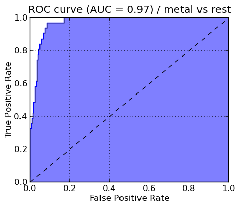
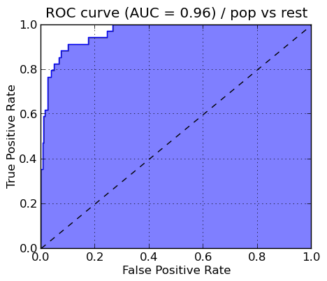
For each selected genre type, a ROC (Receiver Operating Characteristic) curve is generated and stored as a png file in the /graphs directory. The ROC curve is created by plotting the fraction of true positives out of the total actual positives (True positive rate) vs. the fraction of false positives out of the total actual negatives (False positive rate), at various threshold settings.
Some of the sample graphs are shown below alongwith their proper interpretation.
ROC curve of METAL genre
ROC curve of POP genre
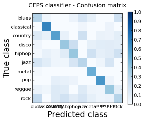
To judge the overall performance, a confusion matrix is produced. A confusion matrix is a specific table layout that allows visualization of the performance of an algorithm. Each column of the matrix represents the instances in a predicted class, while each row represents the instances in an actual class.
The confusion matrix with all the genres selected is shown below.
A spectrogram is a visual representation of the frequency content in a song. It shows the intensity of the frequencies on the y axis in the specified time intervals on the x axis; that is, the darker the color, the stronger the frequency is in the particular time window of the song.
Sample spectrograms of a few songs from the GTZAN dataset.
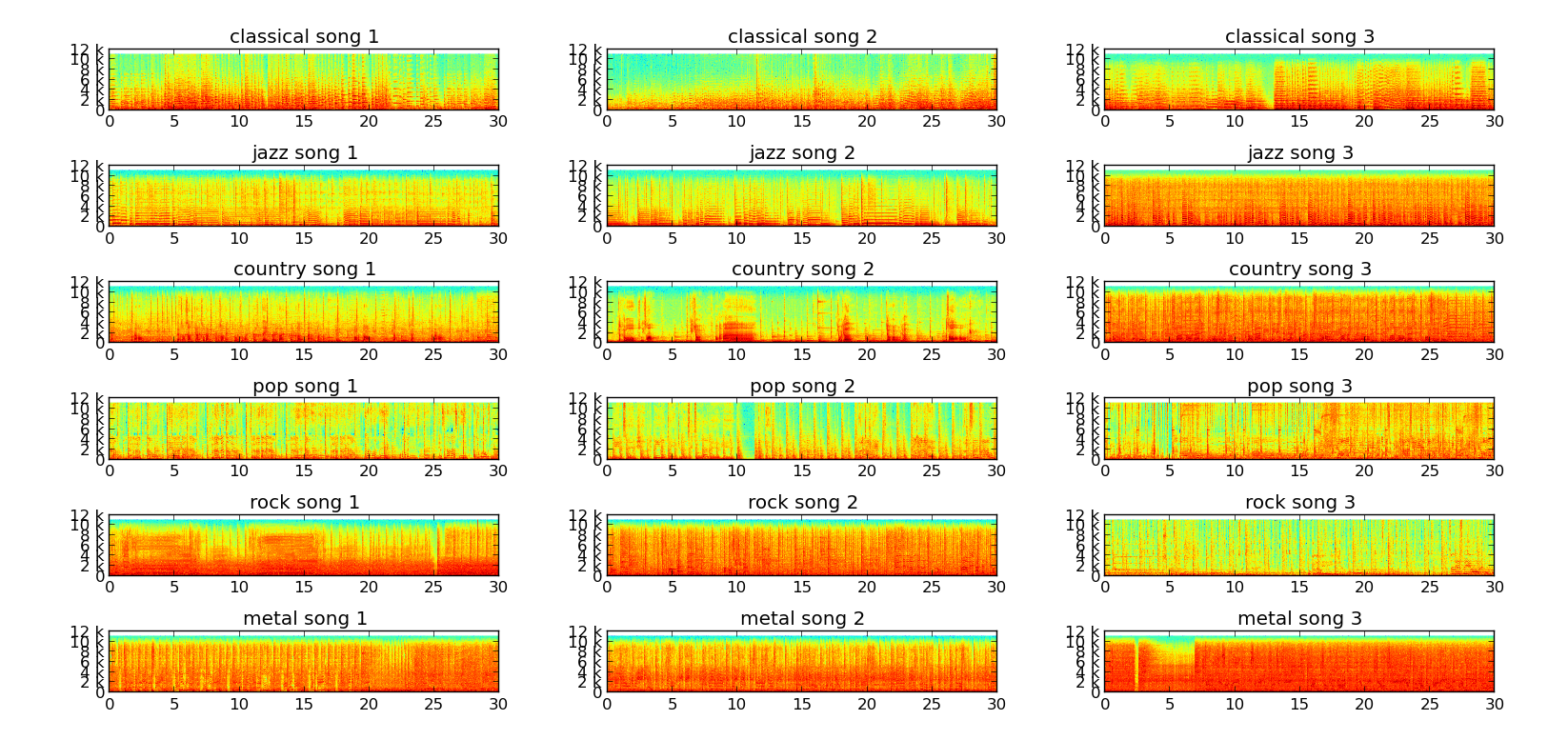
It can be clearly seen from the above image that songs belonging to the same genre have similar spectrograms. Keeping this in mind, we can easily design a classifier that can learn to differentiate between the different genres with sufficient accuracy.
MFCC = Mel Frequency Cepstral Coefficients
The Mel Frequency Cepstrum (MFC) encodes the power spectrum of a sound. It is calculated as the Fourier transform of the logarithm of the signal's spectrum. The Talkbox SciKit (scikits.talkbox) contains an implementation of of MFC that we can directly use. The data that we feed into the classifier is stored as ceps, which contain 13 coeffecients to uniquely represent an audio file.