Forced Homogeneous Isotropic Turbulence
In this tutorial, the setup of a statistically stationary turbulent simulation in a three-dimensional domain is demonstrated. This is a viscous, single-species problem with subgrid-scale stress and heat flux. The following capabilities of HAMeRS will be shown:
- Kinetic-energy-preserving scheme with 13-point fourth order accurate dispersion-relation-preserving finite differencing
- Subgrid-scale model with midpoint diffusive/viscous flux reconstructor
- Special source term for forcing with the use of monitoring statistics
The linear forcing is used for the turbulent kinetic energy production and the Vreman's subgrid-scale viscosity is used for the turbulent kinetic energy dissipation. The ratio of specific heats is 5/3. The problem has a size of [0, 2π)3. This is an incompressible problem as the mean pressure is chosen to be very large.
The kinetic-energy-preserving scheme follows:
Pirozzoli, Sergio. "Generalized conservative approximations of split convective derivative operators." Journal of Computational Physics 229.19 (2010): 7180-7190.
And the 13-point fourth order accurate dispersion-relation-preserving finite difference scheme follows:
Bogey, Christophe, and Christophe Bailly. "A family of low dispersive and low dissipative explicit schemes for flow and noise computations." Journal of Computational physics 194.1 (2004): 194-214.
The file containing the initial conditions of this problem (HomogeneousIsotropicTurbulence3D.cpp) can be found in problems/Navier-Stokes/initial_conditions and the initial conditions should be set up by ln -sf <absolute path to HomogeneousIsotropicTurbulence3D.cpp> src/apps/Navier-Stokes/NavierStokesInitialConditions.cpp. The code has to be re-compiled after the link to the actual initial condition file is set.
The file containing the special source terms of this problem (HomogeneousIsotropicTurbulence3D.cpp) can be found in problems/Navier-Stokes/source_terms and the initial conditions should be set up by ln -sf <absolute path to HomogeneousIsotropicTurbulence3D.cpp> src/flow/flow_models/FlowModelSpecialSourceTerms.cpp.
Since our problem is viscous, we first set the application type to be Navier-Stokes:
Application = "Navier-Stokes"
The next thing to set is the block NavierStokes:
NavierStokes
{
    // Name of project
    project_name = "3D HIT"

    // Number of species
    num_species = 1

    // Flow model to use
    flow_model = "SINGLE_SPECIES"

    Flow_model
    {
        // Equation of state to use
        equation_of_state = "IDEAL_GAS"

        Equation_of_state_mixing_rules
        {
            species_gamma = 1.666666666666667
            species_R = 287.142857143
        }

        // Equation of shear viscosity to use
        equation_of_shear_viscosity = "CONSTANT"

        Equation_of_shear_viscosity_mixing_rules
        {
            species_mu = 0.0
            species_M = 1.0
        }

        // Equation of bulk viscosity to use
        equation_of_bulk_viscosity = "CONSTANT"

        Equation_of_bulk_viscosity_mixing_rules
        {
            species_mu_v = 0.0
            species_M = 1.0
        }

        // Equation of thermal conductivity to use
        equation_of_thermal_conductivity = "PRANDTL"

        Equation_of_thermal_conductivity_mixing_rules
        {
            species_c_p = 1005
            species_Pr = 0.72
            species_M = 1.0
            species_mu = 0.0

            equation_of_shear_viscosity = "CONSTANT"
        }

        use_subgrid_scale_model = TRUE

        Subgrid_scale_model
        {
            subgrid_scale_model = "VREMAN"
            constant_sgs = 0.06
            species_Pr_t = 0.90
            species_c_p  = 1005
        }

        monitoring_statistics_names = "KINETIC_ENERGY_AVG", "MACH_NUM_MAX"
        monitoring_time_step_interval = 1

        has_source_terms = TRUE
        Source_terms
        {
            has_special_source_terms = TRUE
            special_source_box_lo = 0, 0, 0
            special_source_box_hi = 6.283185307179586, 6.283185307179586, 6.283185307179586
            forcing_rate = 0.0001
        }
    }

    // Convective flux reconstructor to use
    convective_flux_reconstructor = "KEP"

    Convective_flux_reconstructor
    {
        use_DRP4 = TRUE
        stencil_width = 13
    }

    use_conservative_form_diffusive_flux = TRUE

    // Diffusive flux reconstructor to use
    diffusive_flux_reconstructor = "MIDPOINT_SIXTH_ORDER"

    Diffusive_flux_reconstructor{}
}
It can be seen that in the Flow_model section, a use_subgrid_scale_model is set to TRUE to turn on the subgrid-scale model and the settings of the subgrid-scale model is set inside Subgrid_scale_model. In this example, the Vreman's subgrid-scale model is chosen with constant turbulent Prandtl number. All physical transport coefficients are set to zero. The monitoring statistics are also chosen including KINETIC_ENERGY_AVG which are required in the special source terms for computing the forcing.
Midpoint diffusive/viscous flux reconstructors with different formal order of accuracy can also be used:
| Settings | diffusive_flux_reconstructor |
constant_sgs |
Formal order of accuracy |
|---|---|---|---|
| 1 | "MIDPOINT_SECOND_ORDER" | 0.10 | 2 |
| 2 | "MIDPOINT_FOURTH_ORDER" | 0.07 | 4 |
| 3 | "MIDPOINT_SIXTH_ORDER" | 0.06 | 6 |
The following settings are used for CartesianGeometry:
CartesianGeometry
{
    // Lower and upper indices of computational domain
    domain_boxes = [(0, 0, 0), (63, 63, 63)]
    x_lo         = 0.0, 0.0, 0.0                                              // Lower end of computational domain
    x_up         = 6.283185307179586, 6.283185307179586, 6.283185307179586    // Upper end of computational domain

    // Periodic dimension. A non-zero value indicates that the direction is periodic
    periodic_dimension = 1, 1, 1
}
The following settings are used for RungeKuttaLevelIntegrator and TimeRefinementIntegrator:
RungeKuttaLevelIntegrator
{
    cfl                      = 1.5e0 // Max cfl factor used in problem
    cfl_init                 = 1.5e0 // Initial cfl factor
    lag_dt_computation       = FALSE
    use_ghosts_to_compute_dt = TRUE
}

TimeRefinementIntegrator
{
    start_time           = 0.0e0   // Initial simulation time
    end_time             = 4.0e2   // Final simulation time
    grow_dt              = 1.0e0   // Growth factor for timesteps
    max_integrator_steps = 1000000 // Max number of simulation timesteps
}
Other unmentioned sections are similar to previous tutorial cases particularly the inviscid Taylor Green vortex problem.
To run the simulation with one core, first put the input file inside a directory named tutorial_07 under HAMeRS. Then, execute the built main executable inside build/src/exec/main with the input file:
../build/exec/main <input filename>
To run the simulation with multiple cores, you can try mpirun/mpiexec/srun, depending on the MPI library used for the compilation of HAMeRS. For example, if mpirun is used:
mpirun -np <number of processors> ../build/src/exec/main <input filename>
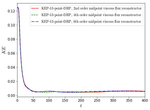
These are the time histories of the kinetic energy with diffusive_flux_reconstructor equal "MIDPOINT_SECOND_ORDER", "MIDPOINT_FOURTH_ORDER", and "MIDPOINT_SIXTH_ORDER" respectively:
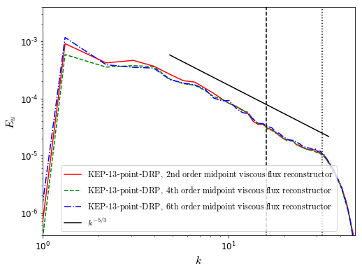
These are the spectra of the x-component of velocity using different settings:
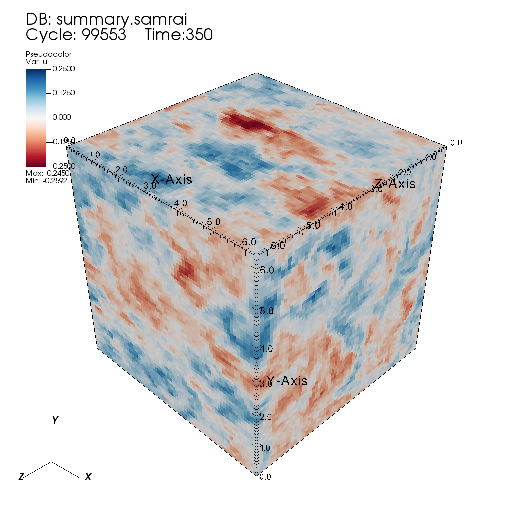
The instantaneous snapshot of x-component of velocity using the sixth order midpoint diffusive/viscous flux reconstructor is shown below: