-
Notifications
You must be signed in to change notification settings - Fork 2
Home
The application is designed as a GUI tool for Continuous pi-calculus (CPi). It is a stand alone program made in Haskell for editing and analysing models written in CPi.
The tool utilizes functionality included in the CPi library from the Command line based tool for Continuous pi-calculus: The Continuous Pi Work Bench (CPiWB). The source code and more details of this tool, created by Chris Banks, can be found on his web page here.
CPi is a process algebra for modelling the behaviour of biochemical systems created by Marek Kwiatkowski.
CPi expresses the behaviour and variation of chemical species within processes. Examples of these kind of processes include enzyme inhibition or intracellular signalling pathways.
For more in-depth details regarding Continuous pi-calculus please see Marek's thesis here or this paper here.
CPi specifies a series of definitions for the components of a model with two levels of system description. These are broken into Species and Processes.
Species: Individual molecules(such as proteins) with transition system semantics.
Processes: Bulk population(the concentration of each species) converted differential equations
Take this cource code example found in the models folder abcd.cpi:
-- Simple reaction: A + B -> C + D

-- A turns into C
species A(a) = a.C();
-- B turns into D
species B(b) = b.D();
-- C degrades at a rate of 1
species C() = tau<1>.0;
-- D doesn't degrade
species D() = tau<0>.D();

-- The overall process Pi specifies the starting concentration of each species.
process Pi = [1.5] A(a) || [1] B(b) || [0] C() || [0] D()
           : {a-b@1};
In this simple example the Species A converts into C and C then degrades over time. Along side this Species Converts into D thus it can be seen that their concentrations take an almost precise inverse change over time.
The next model takes 3 species Q,P and R. The presence of Q leads to an increase of P. P degrades to zero but has a interaction site. When species R binds with this site it is degraded.
-- Q generates a pulse of P.
-- P has a site suitable for arbitrary interaction.

species Q(p) = tau<5>.P(p);
species P(p) = tau<1>.0 + p(x).x.P(p);

-- R binds to P and can be degraded by it.

species R(r) = {x-u@5, x-d@1} r<x>.(u.R(r) + d.0);

-- Whilst the pulse of P is present, R is degraded, then it flat-lines.

process Pi = [0] P(p) ||[1] Q(p) ||[2] R(r): {p-r@1};
http://mareklab.org/talks/pepa08.pdf
To install the tool you can either download the project as a .zip or clone the repository to a location of your choosing. You will need root access to install CPi-IDE. This repository also contains the command-line tool CPiWB and will install this as well.
There are is a whole host of dependencies all of which will be checked or installed by the install_deps script.
To do this use sudo chmod u+x install_deps.sh to make the dependencies script executable.
Then run this script: sudo ./install_deps.sh.
If the script completes succesfully then run the make command.
This should create both CPi-IDE and CPiWB executables in folder.
The tool has a built in text editor for creating and altering model source code. The editor field includes dedicated CPi syntax highlighting.
Models can be created from scratch by simply typing into the empty editor field. These can be saved by using the Save option in the File menu.
Models can be loaded by choosing the Open option from the File menu. This will present the file chooser window where it is possible to navigate to the desired file.
Species or Processes can also be connected to Biomodels web page. To do this simply enter a special comment --Biomodel <component name> is <Biomodel ID number>. This will present a link in the next section that can be used to open the related page.
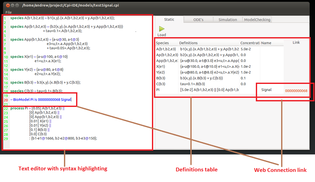
Once the model source code is in the editor the tool can parse this to gain the model definition. This is done by pressing the visible load button.
This will then present the given definitions in the table found on the right hand tab. This allows the model specification to be checked it is as intended.
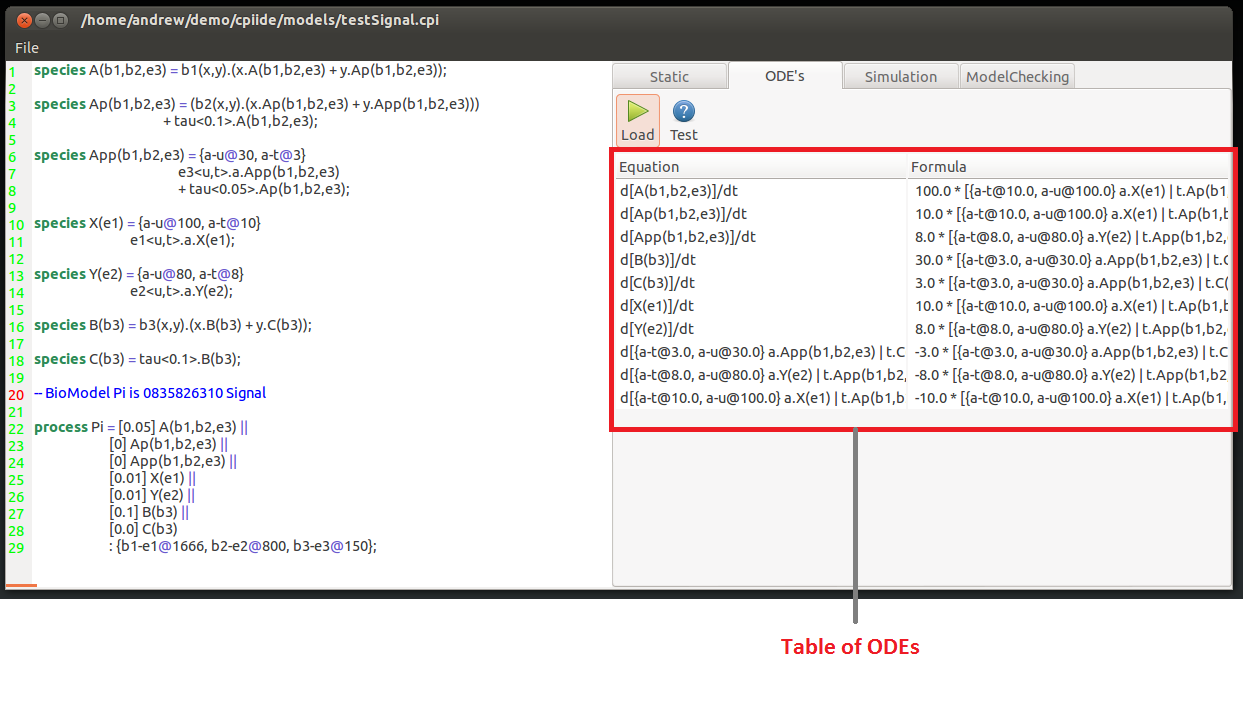
Once you are sure that the specification of the model is correct open the ODE tab.
Here press the Load button will convert the model specification into a series of Ordinary Differential Equations.
At the top of the simulation tab there is a single drop-down menu and 3 entry fields for numerical values.
The drop-down men chooses which process is desired. Then there are 3 entry boxes for:
- Start point of simulation.
- End point of simulation.
- The number visible point between the 2.
Once you have entered the desired values press run. This will display the values of the model components in the table underneath.
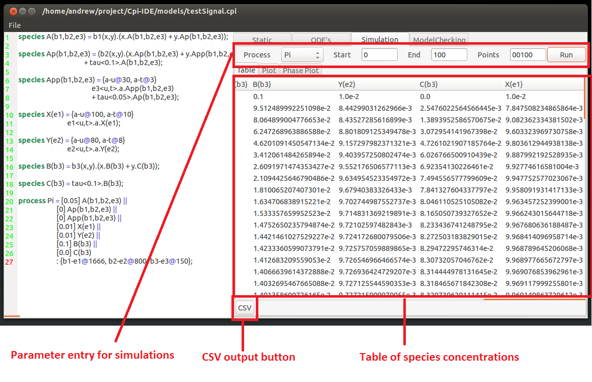
This table of values can be saved to file by clicking the CSV button in the bottom right hand corner. This will open the save CSV window where a name and location of the CSV output file can be specified.
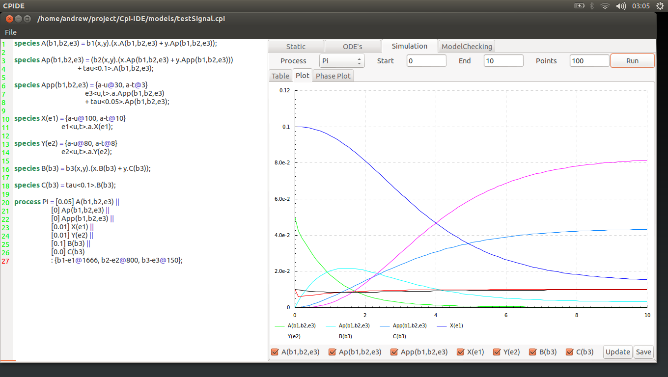
Opening this will reveal a graph showing the concentration of the components plotted for the specified simulation parameters.
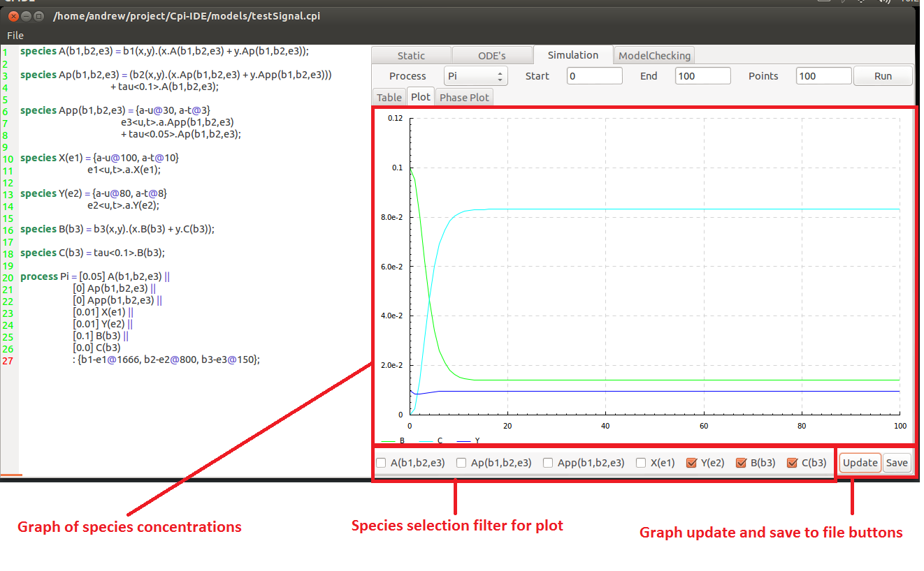
Underneath the graph there are a series of selection boxes that allow the user to specify which of the species they desire on the plot. These changes will not be reflected until the Update button is pressed.
This plot can also be saved to file using the Save button. This will open the save plot window where the location and name of the file is specified.
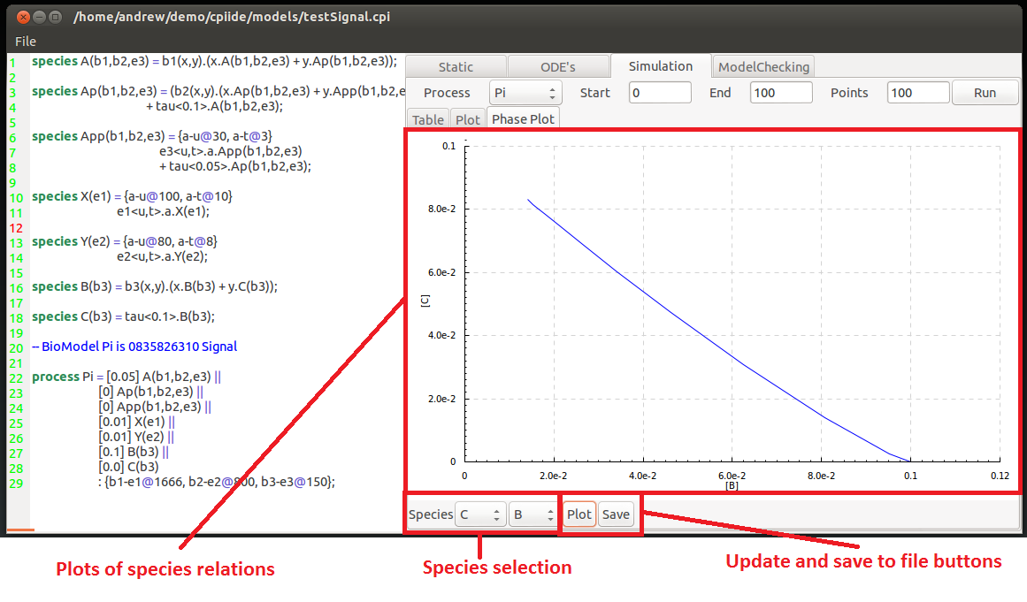
The final tab inside the simulation tab is the phase plot tool. Here two individual different species are picked from the drop down menus at the bottom of the field.
his then displays the relationship of the two species concentrations. Using the value of each of the component as axis it shows what the effect of a higher or lower concentration has on the opposite species, and vice versa.
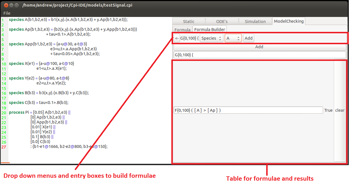
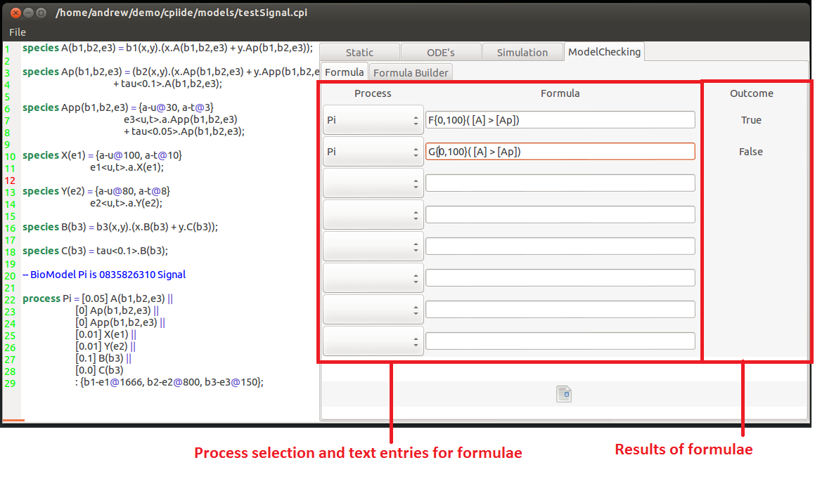
This model checking feature of the tool is a series of entry boxes for logical formulae. This uses the Logic of Behaviour in Context or LBC created by Chris Banks for CPiWB. Individual or nested logical statements can be entered and whether they hold or not can be seen on the right hand side of the window.
To create a formula you need to specify the temporal operator of the hypothesis first.
This can be either:
F{x,y}(Z) Which states that at some point(in the Future) between time-points x & y event Z occurs.
or
G{x,y}(Z) Which states that a all points (Globally) between time-points x & y event Z occurs.
These can be nested to provide more descriptive temporal specifications such as F{0,100}(G(X)) which states at some point condition X is met and holds continuously there onwards.
Within the event there are usual arithmetic and relational operators( +,-, >,=, &,| .....).
The concentrations of species are denoted by square brackets around the species name (concentration of X == [X]).
A more succinct and in depth explanation with further examples of the logic can be found in some of Chris's talkshere and here
The second tab for model checking is the Query builder. This is a series of drop-down menus that will only allow you to add to the formula possible components. This allows users to pick the pieces they desire to build a formula. This can then be checked once it is a acceptable(syntactically correct) formula.
