Demos

mgdemo1

This example shows how you can read video, audio, mocap files into Matlab and how you can preprocess the data. The data is stored as musical gestures data structure after importing. The Musical Gestures Toolbox includes mgdemo1 that contains video, audio, mocap recordings. It is used for the example of this manual. Firstly, read video data into Matlab workspace, mgread can read video, audio, mocap data and create a data structure.

mg = mgread(’pianist.mp4’,’pianist.wav’,’pianist.tsv’)

A musical gestures data structure is imported into Matlab workspace. It shows three substructs, video, audio, mocap, respectively. The video recordings are the pianist who is playing the piano. The length of the video is around 97.5seconds. Let’s further look at the

Figure 1: musical gestures structure

video substruct: Next, we can extract the segment from the structure. For instance:

mgseg = mgvideoreader(mg,’Extract’,10,20);

This operation will extract the length of 20 seconds from 10 seconds to 30 seconds of the video. To keep the same segment with video, it needs to do the same extraction on the audio and mocap data. This can be done by the function mgmap.

mgseg = mgmap(mgseg,’Both’);

Figure 2: video substruct

Alternatively, all operations above can be done by one step. The function mgreadsegment does it.

mgseg = mgreadsegment(mg,10,30);

Sometimes, you may think the video recordings are too large. For instance, the video frame is with 480 by 680 dimension. Usually, this is large enough to satisfy your needs. Downsampling the video may be helpful. The function mgvideosample could help you sample the video conveniently.

mgsam = mgvideosample(mgseg,[2,2],’samplevideo.avi’);

Now, each video frame has been reduced to half. And, the sampled video ’samplevideo.avi’ was written back to disk as well. The sampling factor [2,2] means row and column factors, respectively. If we want to look only the region of interest of the video locally, here mgvideocrop will crop specified region on each frame. The user can define any shape of the region of interest and draw the region on the video frame. The cropped video can be used to compute the motion as well. In a sense, the result should have a good estimation of local objects, such as hands, head, etc. Next, the motiongrams, quantity of motion and centroid of motion can be computed. If the region's position is not given, the user can draw a region, and right-click the mouse and select crop image to create the region.

mgcrop = mgvideocrop(mg);
mgcrop = mgvideocrop(mg,pos);

Figure 3: cropped video

mgsammo = mgmotion(mgsam,’Diff ’);
mgsegmo = mgmotion(mgseg,’Diff ’);

The method ’Diff’ uses the absolute difference between two successive frames. It also provides optical flow method to compute the motion. Furthermore, the function mgmotion could do some filtering operations as well.

mgsegop = mgmotion(mgseg,’OpticalFlow’);

It is interesting to note the player does almost the same action repeatedly from the quantity of motion. From the view of the centroid of motion, most of the blue points cluster in the right side. This is because the player plays the piano using his left hand more often. So the centre of motion appears on the right side. Next, the periodicity of movement might be investigated from the quantity of motion. Let’s have a look at it.

[per,ac,eac,lag] = mgautocor(mgsegmo);

The period is 0.198 seconds. The first maximum at nonzero lag is 0.198 seconds; this is the same as the previous value. Sometimes, it is necessary to show the motiongrams and mocap gram. The function mgvideoplot plots the horizontal and vertical motiongram combined with mocap gram over time.

mgvideoplot(mgsegmo);

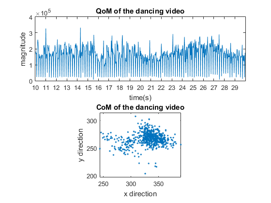
Figure 4: quantity of motion and centroid of motion from 10s to 30s

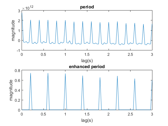
Figure 5: the period estimation of movement

To look at motion more clearly, the vertical motiongram is transposed, and the imagesc function plots the motiongrams after some noise removal. It can be showed that the player repeats a similar action from the horizontal motiongram, which corresponds to the quantity of motion. From the vertical motiongram, it is apparent to note there is only hand playing the piano from 19 seconds to 23 seconds. This explains why most centroid of motion locates on the right side.

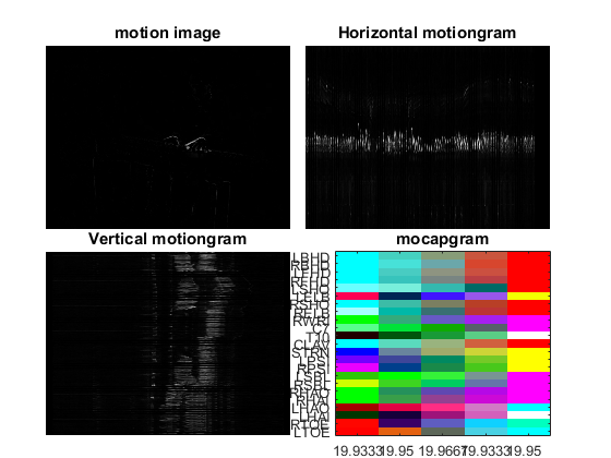
Figure 6: motiongram and mocap gram over time

Figure 7: Horizontal and vertical motiongram, the vertical motiongram is transposed.

Next, let’s continue to investigate the audio recording. mgwaveplot plots the waveform of audio, root mean square and their spectrum.

mgwaveplot(mgsegmo);

Figure 8: waveform, RMS and their spectrum

We may hope that the spectrum of the quantity of motion also gives us some useful information. Here we can compare it with the spectrum of the RMS. Look at the spectrum of QoM; the fundamental frequency is given by 5Hz, which is 0.2 seconds. This value is the same as the period estimated by the mgautocor function.

If we want to look at some motion image features, function mgstatistics can generate first order and second-order features.

features1 = mgstatistics(mgsegmo,’Video’,’FirstOrder’);
features2 = mgstatistics(mgsegmo,’Video’,’SecondOrder’);

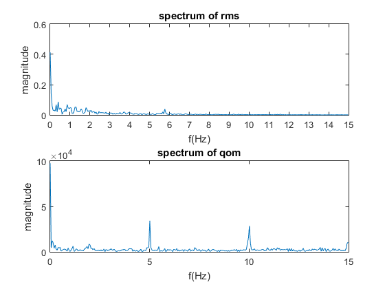
Figure 9: Spectrum of QoM and RMS.

Figure 10: The first order feature space

Figure 11: The second-order feature space

mgdemo2

This example shows how you can read video, audio, mocap files into Matlab and how you can preprocess the data. The data is stored as musical gestures data structure after importing. The Musical Gestures Toolbox includes mgdemo2 that contains video, audio, mocap recordings. It is used for the example of this manual. It extracts 20 seconds from 5 seconds to 25 seconds of the video recording. After this, it should map the same temporal segment to audio and mocap data recording.

mg = mgread(’dance.mp4’);
mgseg = mgvideoreader(mg,’Extract’,5,25);
mgseg = mgmap(mgseg,’Both’,’dacne.wav’,’dance.c3d’);

A musical gestures data structure is imported into Matlab workspace. It shows three substructs, video, audio, mocap, respectively. The video recordings are the nine people dancing to music. The length of the video is around 10 minutes. This demo shows that preprocessing the video recording is very important if the video recordings are quite large. Because the frame size is 1080 by 1920, this is a very high-resolution video recording. In practice, 320 by 480 is enough to compute the motiongram and extract the features. To speed up the calculation, resample the video is necessary.

mgsam = mgvideosample(mgseg,[4,4],’dancesamplevideo.avi’);

The function mgvideosample resamples the video recording. After sampling, the size of each frame is reduced into 270 by 480. Here because of the permission issue, the figure is not shown, we will only show the motion image and motiongram results.

The musical gestures data structure mgsam contains the same temporal segment of the video, audio, and mocap data. Next, you can do analysis based on this data structure.

mgsammo = mgmotion(mgsam,’Diff ’);

The quantity of motion and centroid of motion are shown in the following figures.

Figure 12: Qom and Com of dancing video

The periodicity is estimated by mgautocor based on the quantity of motion. The function waveplot shows the RMS, waveform, spectrogram and spectrum of RMS in one figure.

[per,ac,eac,lag] = mgautocor(mgsammo);

Figure 13: motiongrams of dancing video

mgwaveplot(mgsammo);

In the enhanced period, the first nonzero lag is 0.5 seconds.

It will be interesting to investigate the tempo of the sound and spectrum of the quantity of motion. Here the tempo of the sound can be estimated by function mirtemp in MIR Toolbox. It is 122bpm, namely around 2 beats per second. Figure 15 shows how the QoM changes according to the RMS.

Next, we try to analysis the movements according to the mocap data set. The similarity between 9 persons is calculated by function mgsimilarity in MGT box. However, before computing, the mocap data should be preprocessed. Firstly, take the absolute difference between two successive frames as the way of computing motion image. Secondly, norm the dataset, this is done by function mcnorm in Mocap toolbox.

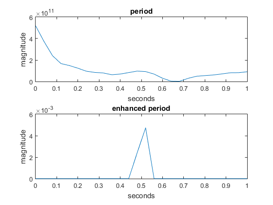
Figure 14: Periodicity estimation of dancing

Figure 15: QoM and RMS

sm = mgsimilarity(mgsammo.mocap.data);

To analyse every person's movements, each person's periodicity of absolute difference movement can be computed in the same way. Figure 19 shows each person’s periodicity of absolute difference movement. From this view, person 2 move to music very regularly.

Figure 16: Plot of the waveform, RMS, and spectrogram of the audio file.

Figure 17: Similarity matrix of 9 persons.

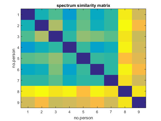
Figure 18: Similarity matrix of the spectrum of 9 persons.

Figure 19: Periodicity of each person.