Undocumented code for personal project on simple recsys via matrix factorization (part 1), and nlp and graph techniques (part 2). Sharing as part of meet-up follow along.
Associated articles:
- Part 1: Building a Strong Baseline Recommender in PyTorch
- Part 2: Beating the Baseline Recommender with Graph & NLP in Pytorch
Talk and Slides:
Electronics and books data from the Amazon dataset (May 1996 – July 2014) was used. Here's how an example JSON entry looks like.
{
"asin": "0000031852",
"title": "Girls Ballet Tutu Zebra Hot Pink",
"price": 3.17,
"imUrl": "http://ecx.images-amazon.com/images/I/51fAmVkTbyL._SY300_.jpg",
"related”:
    { "also_bought":[
		  	"B00JHONN1S",
		  	"B002BZX8Z6",
		  	"B00D2K1M3O",
		  	...
		  	"B007R2RM8W"
                    ],
      "also_viewed":[
		  	"B002BZX8Z6",
		  	"B00JHONN1S",
		  	"B008F0SU0Y",
		  	...
		  	"B00BFXLZ8M"
                     ],
      "bought_together":[
		  	"B002BZX8Z6"
                     ]
    },
"salesRank":
    {
      "Toys & Games":211836
    },
"brand": "Coxlures",
"categories":[
	    [ "Sports & Outdoors",
	      "Other Sports",
	      "Dance"
	    ]
    ]
}
| All Products | Seen Products Only | Runtime (min) | |
|---|---|---|---|
| PyTorch Matrix Factorization | 0.7951 | - | 45 |
| Node2Vec | NA | NA | NA |
| Gensim Word2Vec | 0.9082 | 0.9735 | 2.58 |
| PyTorch Word2Vec | 0.9554 | 0.9855 | 23.63 |
| PyTorch Word2Vec with Side Info | NA | NA | NA |
| PyTorch Matrix Factorization With Sequences | 0.9320 | - | 70.39 |
| Alibaba Paper* | 0.9327 | - | - |
| All Products | Seen Products Only | Runtime (min) | |
|---|---|---|---|
| PyTorch Matrix Factorization | 0.4996 | - | 1353.12 |
| Gensim Word2Vec | 0.9701 | 0.9892 | 16.24 |
| PyTorch Word2Vec | 0.9775 | - | 122.66 |
| PyTorch Word2Vec with Side Info | NA | NA | NA |
| PyTorch Matrix Factorization With Sequences | 0.7196 | - | 1393.08 |
*Billion-scale Commodity Embedding for E-commerce Recommendation in Alibaba
At a high level, for each pair:
- Get the embedding for each product
- Multiply embeddings and sum the resulting vector (this is the prediction)
- Reduce the difference between predicted score and actual score (via gradient descent and a loss function like mean squared error or BCE)
Here's some pseudo-code on how it would work.
for product_pair, label in train_set:
    # Get embedding for each product
    product1_emb = embedding(product1)
    product2_emb = embedding(product2)

    # Predict product-pair score (interaction term and sum)
    prediction = sig(sum(product1_emb * product2_emb, dim=1))
    l2_reg = lambda * sum(embedding.weight ** 2)

    # Minimize loss
    loss = BinaryCrossEntropyLoss(prediction, label)
    loss += l2_reg

    loss.backward()
    optimizer.step()
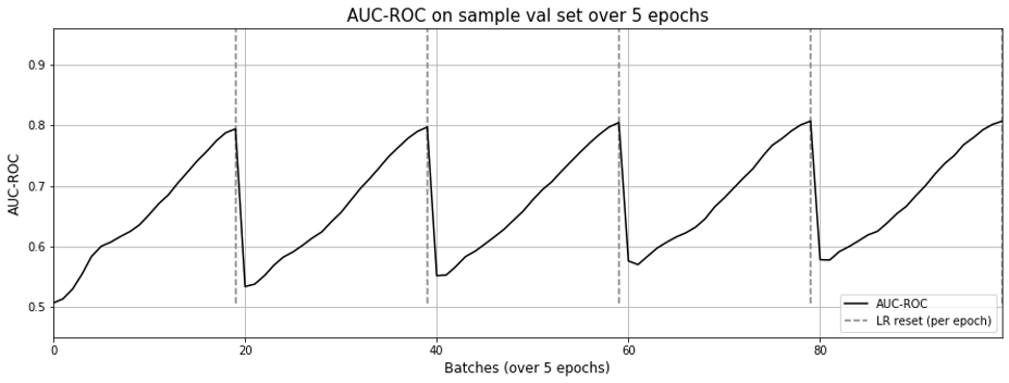
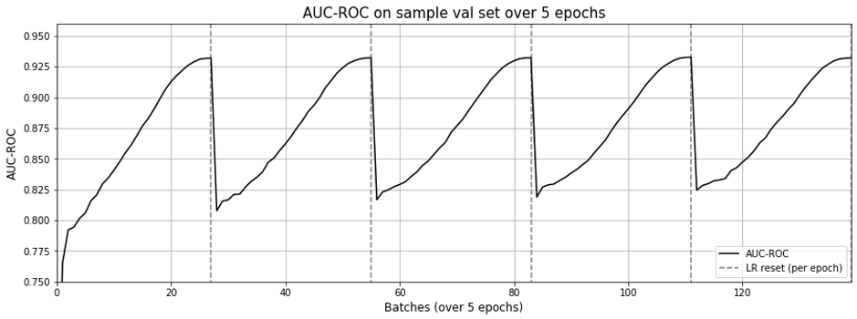
For the training schedule, we run it over 5 epochs with cosine annealing. For each epoch, learning rate starts high (0.01) and drops rapidly to a minimum value near zero, before being reset for to the next epoch.
One epoch seems sufficient to achive close to optimal ROC-AUC.
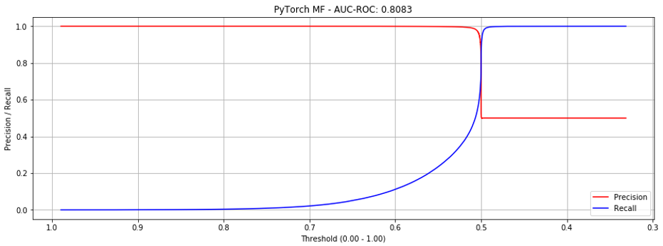
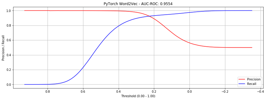
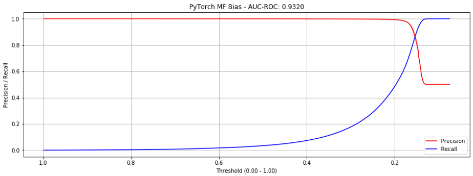
However, if we look at the precision-recall curves below, we see that at around 0.5 we hit the “cliff of death”. If we estimate the threshold slightly too low, precision drops from close to 1.0 to 0.5; slightly too high and recall is poor.
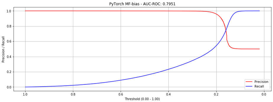
Adding bias reduces the steepness of the curves where they intersect, making it more production-friendly. (Though AUC-ROC decreases slightly, this implementation is preferable.)
I tried using the implementation of Node2Vec here but it was too memory intensive and slow. It didn't run to completion, even on a 64gb instance.
Digging deeper, I found that its approach to generating sequences was traversing the graph. If you allowed networkx to use multiple threads, it would spawn multiple processes to create sequences and cache them temporarily in memory. In short, very memory hungry. Overall, this didn’t work for the datasets I had.
Gensim has an implementation of w2v that takes in a list of sequences and can be multi-threaded. It was very easy to use and the fastest to complete five epochs.
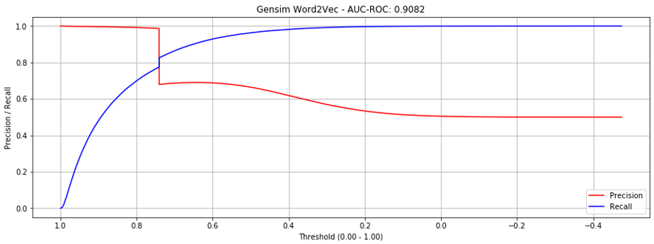
But the precision-recall curve shows a sharp cliff around threshold == 0.73. This is due to out-of-vocabulary products in our validation datasets (which don't have embeddings).
If we only evaluate in-vocabulary items, performance improves significantly.
We implement Skip-gram in PyTorch. Here's some simplified code of how it looks.
class SkipGram(nn.Module):
    def __init__(self, emb_size, emb_dim):
        self.center_embeddings = nn.Embedding(emb_size, emb_dim, sparse=True)
        self.context_embeddings = nn.Embedding(emb_size, emb_dim, sparse=True)

    def forward(self, center, context, neg_context):
        emb_center, emb_context, emb_neg_context = self.get_embeddings()

        # Get score for positive pairs
        score = torch.sum(emb_center * emb_context, dim=1)
        score = -F.logsigmoid(score)

        # Get score for negative pairs
        neg_score = torch.bmm(emb_neg_context, emb_center.unsqueeze(2)).squeeze()
        neg_score = -torch.sum(F.logsigmoid(-neg_score), dim=1)

        # Return combined score
        return torch.mean(score + neg_score)
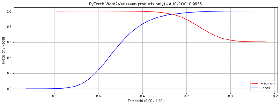
It performed better than gensim when considering all products.
If considering only seen products, it's still an improvement, but less dramatic.
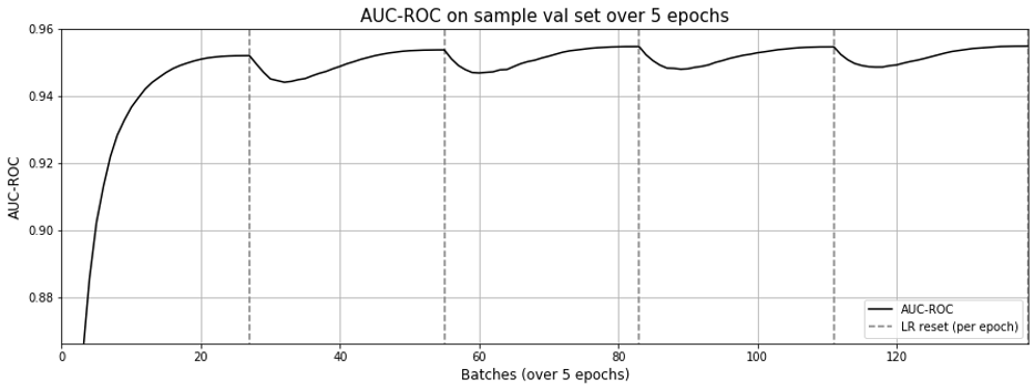
When examining the learning curves, it seems that a single epoch is sufficient. In contrast to the learning curves from matrix factorization (implementation 1), the AUC-ROC doesn't drop drastically with each learning rate reset.
Why did we build the skip-gram model from scratch? Because we wanted to extend it with side information (e.g., brand, category, price).
B001T9NUFS -> B003AVEU6G -> B007ZN5Y56 ... -> B007ZN5Y56
Television    Sound bar     Lamp              Standing Fan
Sony          Sony          Phillips          Dyson
500 – 600     200 – 300     50 – 75           300 - 400
Perhaps by learning on these we can create better embeddings?
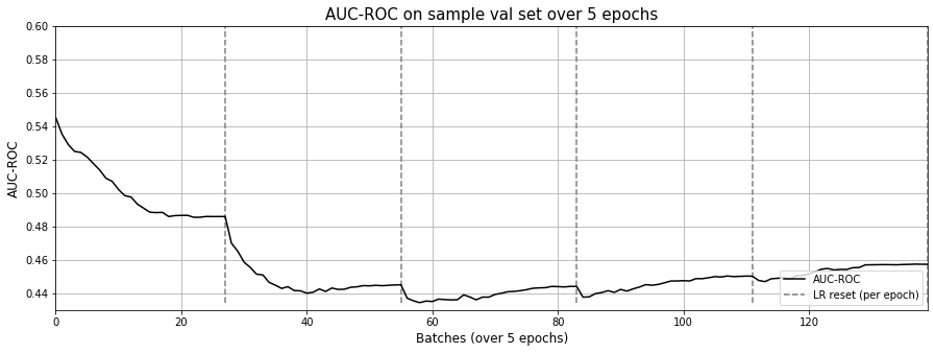
Unfortunately, it didn't work out. Here's how the learning curve looks.
One possible reason for this non-result is the sparsity of the meta data. Out of 418,749 electronic products, we only had metadata for 162,023 (39%). Of these, brand was 51% empty.
Why did the w2v approach do so much better than matrix factorization? Was it due to the skipgram model, or due to the training data format (i.e., sequences)?
To understand this better, I tried the previous matrix factorization with bias implementation (AUC-ROC = 0.7951) with the new sequences and dataloader. It worked very well.
Oddly though, the matrix factorization approach still exhibits the effect of “forgetting” as learning rate resets with each epoch (Fig 9.), though not as pronounced as Figure 3 in the previous post.
I wonder if this is due to using the same embeddings for both center and context.

