The goal of this project is to explore some characteristics of the Budapest Public Transit (BpPT) Network, and compare the network of routes to the network of stops.
The data was downloaded from the BKK Website at 2020.12.15.
To complete this project I used a local PostgreSQL 13 server with DataGrip IDE. DataGrip allows to easily export query as .csv-s, that can be then worked on elsewhere. The Python parts of the projects were also run on a local installation of Python 3 with PyCharm IDE.
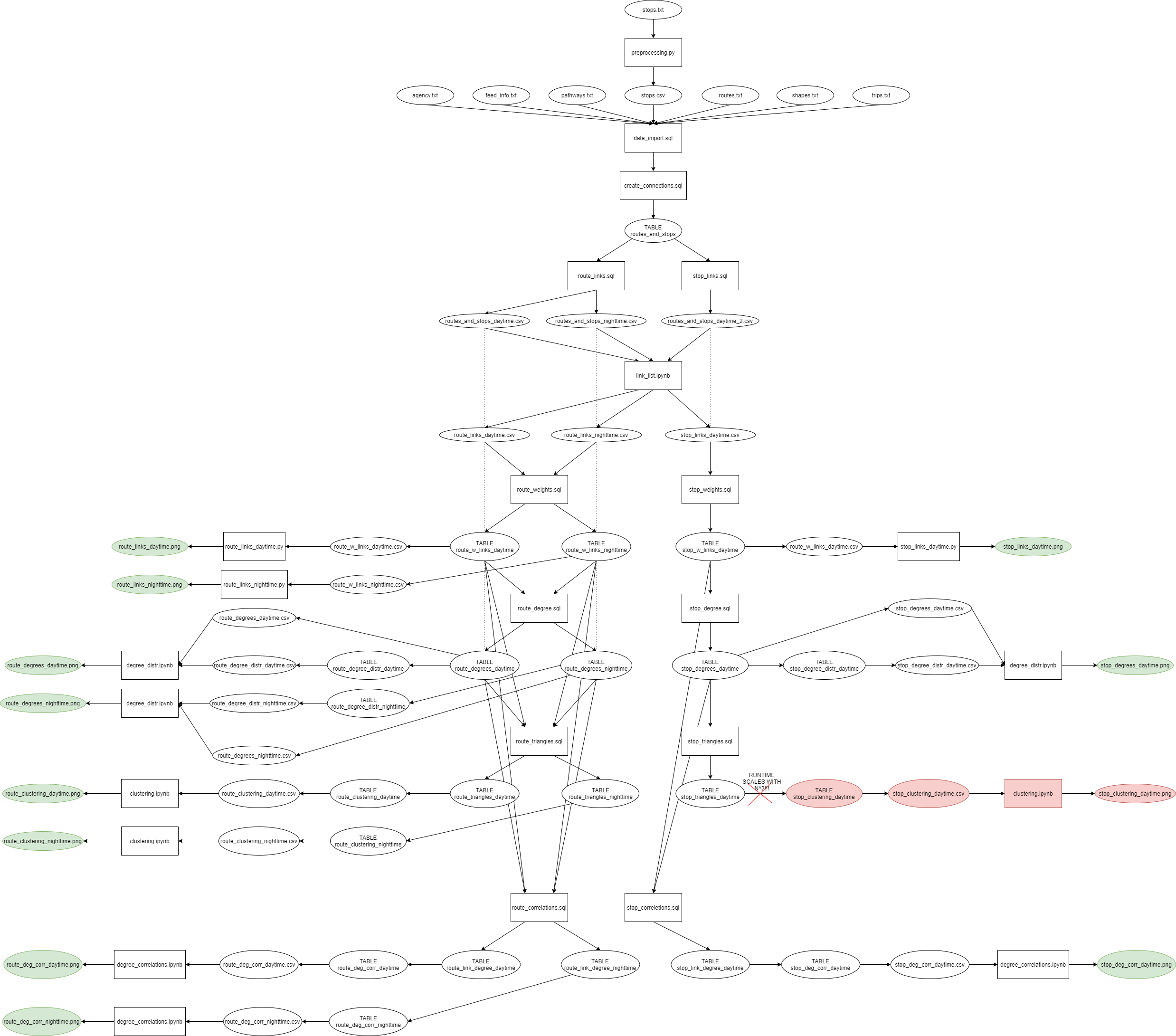
The following flowchart summarizes how the project was done:
It turns out, that within database of stops (stops.txt) some stops have multiple occurrences with nothing linking them together. This happens for example when there is a Metro station named "Sesame Street" and the corresponding bus stop on the surface will be named "Sesame Street M". Thus when trying to evaluate which routes share a stop, this two would be marked as a different stops. (There is no ID linking them, nor do they share a "parent station".) To solve this problem some preprocessing work had to be done. First I went through the database and edited a couple outlier names, that only occurred once, then I loaded in the data to preprocessing.py and with that I removed the "M"-s, "M+H"-s etc. from the stop names. This way the stop name can be used to connect routes. (Even if the ID-s are still mismatched.)
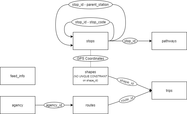
With stops being done, I created a new database named bkk, and with data_import.sql I imported the downloaded data. I did not use the caledar_dates.txt and stop_times.txt as I do not intend to use any temporal data for creating the network. The relationship between the tables is depicted on this chart:
The tables contain the following:
- agency - Basic information about service provider.
- feed_info - Basic information about the feed that is pushed to the BKK Futár service.
- pathways - Contains which stop is connected to which in a route. ("What's the next stop if I'm at X?")
- stops - Contains a list of all the stops with their location(GPS coords.) and other attributes.
- routes - Contains a list of all the routes with their names, short description and color coding for the online map.
- shapes - Contains collections of GPS coordinates, which when drawn on a map will show the shape of the routes used by public transport vehicles.
- trips - Contains which shape corresponds to which route.
Next a table had to be created that contains which stop belongs to which route. This was done in create_connections.sql. The tables "shapes" and "stops" can be joined on the shared GPS coordinates, and then this selection can be joined with "trips" on the shared shape_id-s resulting in a selection that contains the names of the stops, and the routes that use them.
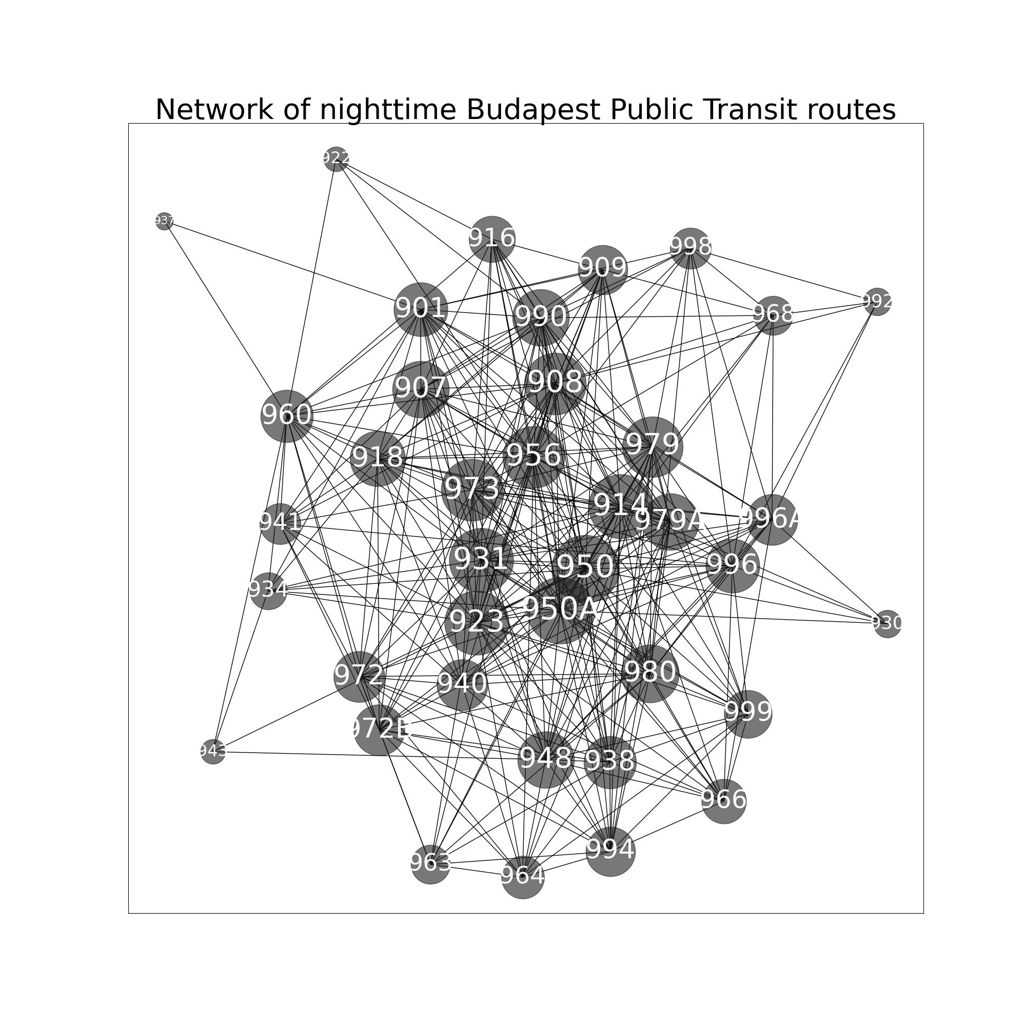
Furthermore this is the point where we let go of the directionality, by assuming that all stops are bi-directional. (~6% of the data violates this assumption.) We'll also split this table in two, having one that contains only the routes of the daytime traffic, and one that only contains nighttime traffic. We do this, because the temporal distance between daytime and nighttime routes is usually measured in hours, and by not doing so we'd essentially make the nighttime buses the most-connected routes in the Network by virtue that they generally use the routes of multiple popular daytime buses. (Not doing so would result in something like this)
To describe a network one has to provide a way to say which node is connected to which. The space efficient way to do this on bigger networks is a link list, where the first column describes the starting node and the secd the destination node of a link. The following linking rules have been used:
- In order for two routes to be connected they have to share at least one stop. (Multiple shared stops warrant no extra link, since that would over-inflate the importance on routes that share a lot of stops. Think tram lines 4 and 6 for example.)
- In order for two stops to be connected you have to be able to go from one stop to another with a single route. (No transfers!)
To create these lists SQL queries are not enough, we can use SQL to order the data in a way that is faster to evaluate within a loop, but using a traditional for loop cannot really be circumvented. (Maybe by using the same number of duplicate tables as the highest number of connections created by a single stop/route, which wouldn't be efficient...) Thus route_links.sql was used to select all stops, that have more than one route attached to them, and order them by the stops. (For the stops network (stop_links.sql) each route has multiple stops attached, so that part of the filtering isn't useful.) By iterating through the resulting selection (link_list.ipynb) only one question had to be asked is the previous stop (or route, for the stop network...) the same as the current one? If the answer is yes, than we just collect the id/name in a list, however if the answer is no, we take the current list and create all possible 2-way permutations and append them to a DataFrame these permutations are the links between the nodes. After that we reset the list, and append the new/name id corresponding to the new stop(or route).
The link list obtained this way has a flaw: It contains multiple identical links, which as I previously mentioned is unnecessary. Using the SELECT DISTINCT query (route_weights.sql;stop_weights.sql) the duplicates are eliminated, and we also add a new column called weight, that only contains "1"-s. This will help in determining the degree distribution later on.
With this, however we have tables, that can be used to plot the network to see the fruit of the work done until this point. This was achieved with the Networkx python library. (route_link_daytime.py;route_link_nighttime.py;stop_link_daytime.py) To calculate favorable positions for the nodes on the plot the Kamada-Kawai algorithm was used.
The results speak for themselves:
What can we gather from these images?
- The better connected and more important routes are at the center, the less connected ones are around the edges. Take a look at for example Route 297 one of the least connected routes placed on the left edge of the network. Or for example the local railway (HéV) lines also tend to be around the edges.
- Notice how the M3 replacement bus is more important, than the operational part of the M3 line. (The replacement bus goes through the city center.)
- An other interesting insight is how tramlines 4-6 are placed near each other (they have very simialr connectedness to the other nodes), or how the tram line 60 (cogwheel-rail) is placed near the buses that go near the Svábhegy-Normafa region.
- On the stops network we can see clear clusters of stops (sadly these can't be labeled in a useful way) belonging to the same routes.
Overall it is nice to see that the intuition is confirmed by these plots. (Well-connected routes going through the city center are more "important" than those near the outer districts...)
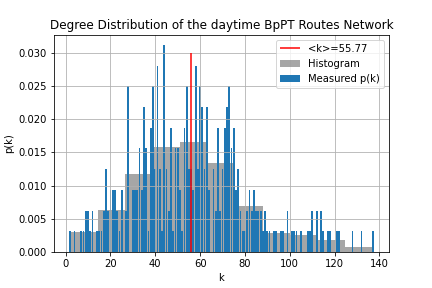
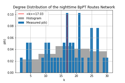
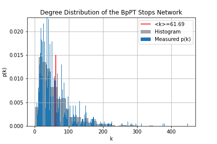
One of the most important properties of any network is its degree distribution. In the case of the "routes network" p(k) gives the probability, that given I'm sitting on a random route what is the chance that I can transfer to k number of other routes? For the "stops network" p(k) answers the question, what is the chance that given I'm at a random stop to be able to go to k number of stops without a transfer?
To obtain these distributions all we need to do, is to count how many nodes are there with k degree. First we should know the degree of each node, this is done through route_degree.sql and stop_degree.sql. Then the simple histogram is made. These don't look attractive, so within degree_distr.ipynb using matplotlib.pyplot.hist() histograms with bigger bin sizes were used, to have a easier to understand figure from the degree distribution. Determining the average degree is just a simple select query, where we take the average of the node degree table.
From these we can tell, that the distribution of the routes is - while not normal - well described by it's average degree, meaning most routes have more-or-less the same number of transfers, with no huge hubs. Contrary to this, the stops have a power-law-like behavior that is not well described by the average degree. We can also tell, that there is a distinct k_min which should correspond to the minimum number of stops it takes to make a route. (Of course this is somewhat contorted by the fact that there are shorter routes, which likely correspond to routes headed for garages and such.) Hub-like behavior also seem to be present here.
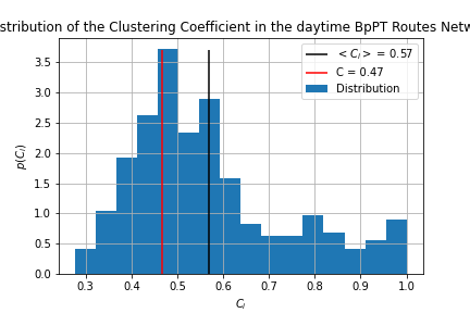
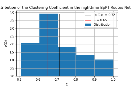
The clustering metric tells us whether the network contains tightly knit groups, however there are two definitions: Global clustering (C) is defined by
Local clustering coefficient tells us how clustered are the nodes near a given node:
Where is the number of links between the neighbors of node i. This also can be translated to how many triangles node i is part of vs. how many it could be part of.
Thus the first aims to make a t able that contains all triangles in the network. (route_triangles.sql,stop_tringles.sql) This is achieved through finding the second neighbors of each node (while making sure the initial node isn't marked as a second neighbor) then getting those third neighbors, which coincide with the initial node completing the triangle. By looking at the length of the list, and calculating the number of possible triangles the global clustering coefficient is obtained. Next to calculate the local clustering I ordered the triangles and counted how many are there for a given node. (Which was then diveded by the num of possible triangles given by the node degree.) This process turned out to scale as
with the number of triangles in the network, which is problematic for the stops network, as it contains over 5 million triangles, and so I did not obtain the local clustering for the stops network, as I'm not comfortable with letting my machine run for roughly 50 hours.
The visualization was done in clustering.ipynb we can see, that the nighttime routes are more clustered, than the daytime ones, and that the global clustering is lower for both cases, than the average local clustering. The global clustering for the stops network was 0.436 making it the least clustered from the three.
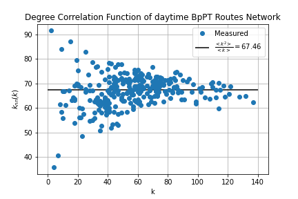
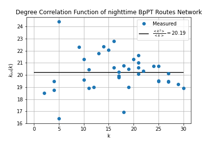
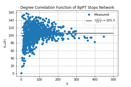
The final metric to be considered in this project is the measuring of degree correlations within a network. Here the question is, whether high degree nodes like to connect to each other, or do they avoid each other?In assortative networks tend to link hubs together, in disassortative networks hubs avoid linking. In neutral networks there is no preference. To measure assortativity we'll use the degree correlation function defined by
Where k-s are the node degrees, and is the adjacency matrix. In a neutral network this function is constant and takes the value
These calculations were carried out within route_correlations.sql and stop_correlations.sql. First I modified the link list table, to contain the degree of the nodes at each end. Since the adjecency matrix is 0 if there is no link and 1 if there is (for unweighted networks) by summing over the degrees on one end for a given node in the modified link list we'll get the same result as and then it just have to be divided by the node degree for the given node. The results were visualized by degree_correlations.ipynb.
Comparing these to the typical example of the different network types it's hard to give conclusive answers on assortativity. We can see, that in the low-k range the degree correlation function fluctuates wildly, while for high k-s it tend to go towards the neutral line.
-
The stops network contains clear clusters/communities that we know correspond to the lines they are part of, with of course one stop being able to be part of multiple lines. (This is often called fuzzy clustering.) Since we have good knowledge on this network it could be used as a benchmark for fuzzy clustering algorithms.
-
The power-law-like behavior of the stops network could be explored further.
-
Could we get a random network that behaves similarly as the routes network?
In this project I showed, how differently a bipartite network's sub-networks behave, and have quite distinct degree distributions, clustering, and degree correlation behavior. It was also advantageous to separate the nighttime routes into a smaller network, as it allowed me to quickly prototype the different queries and code needed to tackle each part.
While a goal of this project is to familiarize myself with SQL in Network Science, there are certain problems that cannot be solved with pure SQL. For this purpose exist procedural languages like "PostgreSQL PL/pgSQL", but using loops within these is as slow as in any other language. And thus for example in Python the usage of robust libraries makes for a more efficient workflow, than trying to implement something in PL/pgSQL. I strived to use SQL for it's strengths in this project, while patching its shortcomings in Python.
Of course in the future it's better to use SQL through Python (multiple packages available for that purpose), and that wouldn't require to save queries and load them in a .py, resulting in a confusing mess of files...
-
Data - From the BKK Website
-
Albert-László Barabási: Network Science
