This is a collection of MATLAB functions and classes designed to provide basic orbital analysis capabilities. This toolbox is intended for users seeking quick and easy calculations which may act as a starting point for mission planning, however, this toolbox would be insufficient for a comprehensive mission design.
This README outlines some of the key features and methodologies implemented in this toolbox. Specific documentation and assumptions are outlined in the relevant function documentation found in the source code or by using the MATLAB help command. For examples of various use cases see the orbital-toolbox/example_usage/ directory.
This toolbox is based on code originally developed for a University of Sydney assignment in the Space Engineering 1 course (2017 Semester 2). The code has since been refactored for use in more general cases, while some of the original tasks are still shown as example usage.
- Clone this repository to your local machine using one of the following:
git clone [email protected]:MatthewSuntup/orbital-toolbox.git
git clone https://github.com/MatthewSuntup/orbital-toolbox.git
- Navigate to the directory where you cloned the repository in MATLAB's file tree
- Right click on the
orbital-toolboxdirectory and selectAdd to Path -> Selected Folders and Subfolders - Call the desired functions in new scripts or modify the scripts in the
orbital-toolbox/example_usage/directory
The tle(line_1, line_2) function takes two strings corresponding to the first and second line of a two-line element (TLE) set and returns a map of key-value pairs for each element. The toolbox provides a Satellite class with the method Satellite.updateFromTLE(tle_file) which utilises this function and then stores the map data into properties of the Satellite object.
Additional orbital parameters may be calculated from the TLE data using the Satellite.updateOrbit() method of a Satellite object. This method will analytically determine the following values, using the formulae outlined here:
where is the mean motion.
where is the period,
is the gravitational constant, and
is the mass of the Earth.
where is the semi-major axis, and
is the eccentricity.
where is the semi-major axis, and
is the radius of perigee.
where is the radius of apogee and
is the radius of perigee.
These values are stored in an Orbit object which is a property of the Satellite. Once these parameters have been a calculated, an Orbital Simulation is also run.
The Orbit.sim() method is provided by the Orbit class and generates an array of mean anomaly values, true anomaly values, radial distances, and cartesian coordinates, corresponding to a complete orbit. The data may be used for further analysis, polar plotting, or cartesian plotting. The method performs the following calculation:
- Generate an array of linearly spaced mean anomaly values
- Convert these values to eccentric anomaly vales using the Newton-Raphson method to solve Kepler's equation:
- Convert eccentric anomalies to true anomalies:
- Calculate the radial distance:
This resulting data is compared against the known semi-major and semi-minor axes to obtain the simulation error.
The Orbit.plotOrbit() function provides a quick method of plotting a simulated orbit using a cartesian or polar plot.


The Orbit.pathArea() method simply calculates the area of the orbit using:
where is the semi-major axis and
is the semi-minor axis.
The Orbit.pathLength() method approximates the line integral of an ellipse to find the length of the orbit. The path length is given by:
where is the eccentricity of the orbit.
In order to evaluate this computationally, the formula implemented in this toolbox is:
The program will continue to loop until the increment added by the successive term is less than 100m, as the error at this point will be less than that associated with the semi-major axis.
The maxViewTimeStat(Ro, visible_ang) function will calculate the maximum length of time a satellite in a circular orbit will be visible from the ground when passing directly overhead through the zenith of the observer, given a minimum viewing above the astronomical horizon. By assuming a circular orbit, spherical Earth, and stationary (non-rotating) Earth, it is possible to calculate this analytically using only the orbital radius and viewing angle (in the following diagrams the viewing angle is noted as being 5°, however, the illustration is exaggerated).

To get the viewing time for non-zenith passes, use the viewTimeStat(Ro, visible_ang) function, which will generate an array of maximum elevation angles and corresponding viewing times (where an elevation of 90° corresponds to a zenith pass).

An example of the results obtained for an observer able to see 5° above the ascending and descending horizon, viewing a satellite at an altitude of 590km is shown below:

Note that running the maxViewTimeStat(Ro, visible_ang) function with the same input arguments will return the singular value of 618.5 seconds, seen in this graph as the viewing time for an elevation of 90°.
The previous functions assumed a stationary Earth, this makes the calculation significantly less computationally expensive, and requires minimal information about the orbit and observer. The viewTimeRot(Ro, i, visible_ang, loc) function using a computational method to achieve an equivalent result, but this time taking into account the rotation of the Earth.
The concept driving this approach is that the longitude and latitude of the ground station may be converted to Earth-Centred Earth-Fixed (ECEF) coordinates, while the Satellite's movement in the perifocal plane is also converted to ECEF co-ordinates. The condition for the satellite to be visible is simply that it must be closer to the ground station than the distance associated with the edge of its cone of view. The simulation iterates through a set of varying RAAN values, and checks for this condition at each point along the orbit. The maximum elevation is then calculated from the closest point of the approach.
An example of the results obtained for an observer standing at Sydney Observatory, able to see 5° above the ascending and descending horizon, viewing a satellite at an altitude of 590km and inclination of 97°, is shown below:
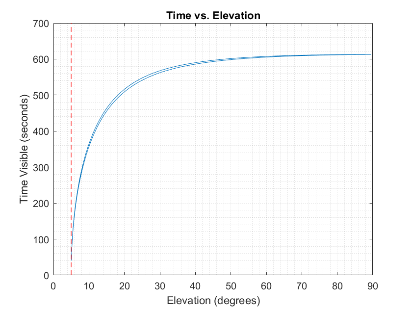
Note that when the rotation of the Earth is considered, the time of visibility is shorter (612.5 seconds at 90° elevation in comparison to the previous 618.5 seconds). Additionally, there is an asymmetry between elevations on the east side of the zenith and the west side (seen in the offset blue line).
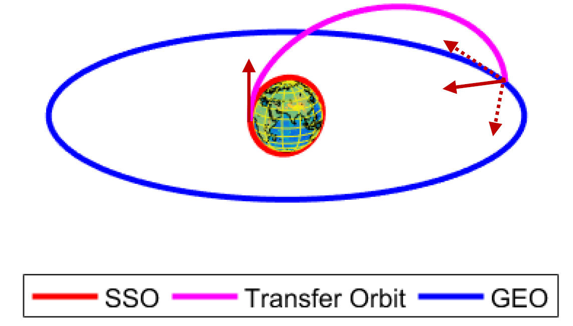
The hohmann(r1, r2, theta) function calculates the required changes in velocity at the perigee and apogee of a transfer orbit for a Hohmann transfer between two circular orbits. The calculations used by this function assume that the burns are instantaneous, and that the eccentricities of the starting and final orbits are 0. Additionally, it is assumed that the inclination change is to occur entirely as part of the second burn, so the second burn is effectively a vector sum of a burn to circularise the orbit and a burn to change the inclination.
The semi-major axis of the transfer orbit is given by:
The velocities associated with the initial and final orbits are given by:
The velocity at the perigee and apogee of the transfer orbit is given by:
where for the perigee and
for the apogee.
Finally, the delta-v value at perigee is given by:
where is the difference in inclination between the two orbits.
For example, we can find the delta-V necessary to move the ESA's PROBA1 satellite from its current orbit with an inclination of 97.6° and an altitude of 585km, to a geostationary orbit with an inclination of 0° and altitude of 3579km. This function tells us that the required delta-V at the perigee of the transfer orbit will be 2347 m/s and the required delta-V at the apogee will be 3668 m/s.
The launchAzimuth(i, r, lat, inertial) function calculates an appropriate launch azimuth for a rocket to reach an orbit with a given inclination and radius, from a launch site at a given latitude. First, the function finds the inertial azimuth, that is, the launch azimuth that would be used if the starting velocity associated with the rotation of the Earth was neglected.
where is the inclination of the destination orbit, and
is the latitude of the launch site.
It is assumed that the launch is directed eastwards (in the same direction as the Earth's rotation, to conserve energy). Taking into account the effects of the rotation of the Earth, the launch azimuth becomes:
For example, if we want to launch a rocket from the Guiana Space Centre to an orbit with an inclination of 56° and altitude of 300km, this function tells us that the desired launch azimuth would be 31.2°.
In-orbit RAAN changes can be very fuel inefficient and are often unnecessary if the correct launch time is chosen for a desired RAAN. The launchTime(RAAN, i, r, loc) function calculates a possible launch time in order to launch directly into an orbit with a given inclination, RAAN, and orbit radius, from a given launch location (assuming an appropriate launch azimuth is used, see Launch Azimuth). Note that the desired launch time will repeat every sidereal day, and so the launch time provided is simply the next available opportunity after the 2020 March Equinox and a user may add or subtract an integer number of sidereal days to find the launch time on any desired day. The time provided and location taken by this function are that of burnout, as it does not account for the mission-specific dynamics associated with the rocket, however, we will assume that burnout occurs instantaneously, allowing us to refer to the launch time and location.
The function first calculates the difference in longitude between the burnout location and the ascending node, using the formula:
where is the latitude of the burnout location.
Consider the Earth in an Earth Centred Inertial (ECI) reference frame, in which it is rotating beneath the stationary vernal equinox. To find the launch time, we want to find how long it will take for the planned location of the ascending node to rotate from its position at the time of the March Equinox to the vernal equinox. If we consider the longitudes to be expressed in terms of 0 to 360° from the prime meridian to the East, then we can express the angle that the Earth must rotate as:
in the ECI reference frame, we take Earth's rotation to be one sidereal day, and so the time between the March Equinox occurring and launch can be expressed as:
where is the length of time in a sidereal day. This time is then added to the time of the March Equinox (in 2020, this occurred at 03:48 on the 20th of March (UTC)).
For example, if we want to launch into an orbit with a 56° inclination, 300km altitude, and RAAN of 317°, from the Guiana Space Centre, this function tells us that the first available time after the 2020 March Equinox to do so will be on the same day at 12:59:39 (UTC).
When I originally developed much of this code in 2017, I researched the relevant space engineering concepts and gained a fundamental understanding of the orbital dynamics associated with the functionality of this toolbox. Returning to this project in 2020, to refactor and develop it into something more re-usable, gave me a welcome refresher on fundamental orbital dynamics and MATLAB programming.
Thank you to the University of Sydney for the original task specifications which inspired the creation of this toolbox, and to my classmates who kept me going through all the late nights while working on this originally.
Space Mission Analysis and Design: The New SMAD, James R. Wertz (2011) was the main source of reference for all of the formulae outlined in this README and implemented in the toolbox.
This work is entirely my own and has been modified since it was originally implemented for an assignment. It should not be copied in any form by students in university courses with similar assignments. If you are struggling with a similar project and want to get in touch I would be happy to have a chat and help out with your understanding or point you to some useful resources!