
-
app: It includes the application code in streamlit, as well as the previously trained model.
-
data: It contains the original dataset and the clean dataset, that is, where we preprocessed outliers.
-
doc: Documentation in pdf.
-
src: Steps for creating the model and the application.
- Age of the insured.
- BMI body mass index.
- Children Number of children of the insured.
- Region User's place of residence.
- Smoker Whether the user smokes or not.
- Charges Health insurance price.

When performing a histogram, we notice the presence of atypical values, that is, values that are out of the norm.
We deduce that these values can have a better explanation if we add more variables.
We create a box and whisker plot where we add the variable smoker. We discovered that it is a variable that greatly influences the price of health insurance.
We also found that if the user is a smoker and has an advanced BMI. The insurance charge increases more, since the insured will have more charges due to his state of health.
The BMI maintains a linear trend relationship compared to the predicted insurance. That is, one value increases proportionally to the other.
We observe 4 "clusters":
-
The first is for healthy people who do not smoke are healthy, as a consequence they do not have severe medical problems.It maintains a linear relationship with age, that is, age is proportional to medical position.
-
People who do not smoke but have significant health problems.
-
People who smoke but have a good health condition.
-
Users who smoke and have serious medical problems.
It can be simplified under two conditions. The first where the condition is not so serious and the second is when the case is dedicated.
We could create an additional feature, to be able to classify users based on the degree of health of the user. Since, as we can see in the graph, the quality of health influences the medical position.
-
The variables that refer to describe some habits and characteristics of users influence the insurance charge.
-
We discovered a new hidden characteristic in the dataset when comparing age with the price of insurance based on whether the user smokes or not, we could add another new variable to the problem that refers to the degree of the health problem.
Feature engineering consists of dealing with missing values, outliers or creating new important variables. Where an optimal treatment for such data is found, this step is very important for the performance of the model. Since it is the data that we are going to give to train the model.
We decided to separate the data into smokers and non-smokers, with the aim of giving the data a better treatment.
We apply the central limit theorem, which is a technique used to establish confidence intervals. We use these intervals to create a new important feature, which can explain the outliers.
We apply intervals to group based on the cost of health insurance. We divide them into people with less serious medical problems and people with severe medical problems.

For both models, we use the same variables. We apply data rescaling process, although for assembly models it is not necessary. Since these algorithms work through decision trees, they use mathematical inequalities.
We do not discriminate any variable, although in the EDA. We found that the variables smoker, age and bmi influence the cost of health insurance.
Although it could eliminate variables such as gender and region. I didn't want to remove it as the difference between humans and algorithms. It is that we take the most important variables, while the algorithms use these variables and complement them with other variables in which they find unknown patterns. They favor the quality of the prediction.
We create 3 regression algorithms:

A simple linear regression consists of finding the best straight line that fits the set of data.
Its mathematical formula is the following:
-
$y$ the variable to predict -
$x$ represents the variable -
$x$ the weight of the coefficient -
$b$ the intercept
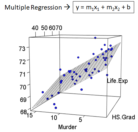
But in this case we will use a multiple linear regression model, where the best hyperplane that fits the data will be found. Because we are dealing with 2 or more predictor variables.
The formula is very similar to the simple one with the difference that more coefficients are added accordingly to the number of variables.
It has the advantage that it is easy to interpret. It has the disadvantage of requiring a scale adjustment so that the variables can be compared with each other.
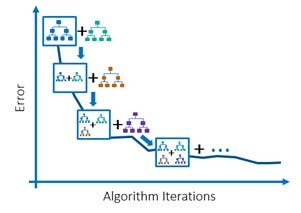
Gradient Boosting and XGBoost are some algorithms that belong to this category. These algorithms work using weaker algorithms, usually decision trees. That each time they are improving with respect to the learning rate and the number of estimators,one of the main differences is that XGBoost can be executed through a GPU, something that allows faster training.
We use the same parameters for XGBoost and Gradient Boosting.
- max_depth: It refers to the maximum depth of the decision tree. For the first evaluation we use a maximum depth of 2 and in the second of 3.
- n_estimators: Number of decision trees. The range of estimators we used was from 100 to 1000.
- learing_rate: It is the room for improvement for each iteration. We use a learning rate of 0.01

-
Underfitting: It is due to the lack of variables; therefore, it does not perform well with training and validation data.Due to the lack of variables to consider.
-
Perfect Fit: The model yielded excellent results for both the training and validation data.
-
Overfitting: Occurs due to outliers and an excessive number of variables. where the model performs well for the training data. But it is unable to adapt to data that it has never seen.

It consists in finding the ideal number of estimators. Since it makes no sense to use more estimators, if the validation data is not there is a drastic improvement.
It measures the average error between the value predicted by the model and the original value.


The 3 models are learned to solve the problem. But the most complete model is XGBOOST, since it has a squared error with respect to its competitors.
It has the advantage that it does not need a scale adjustment for numerical variables, it uses the original values since it works based on mathematical inequalities.

The most significant variables are smoker and medical problem. Since people with severe problems, the medical cost is much higher than that of a healthy person.
XGBOOST offers outstanding performance, generalizes very well, easily accomplishes the task of providing robust predictions.
As a curious fact, this type of model is the winner of multiple competitions in Kaggle, which is a kind of social network for data scientists.
https://jesus-vazquez-a-insurence-app-streamlit-app-insurence-rbv8gd.streamlitapp.com/