Vehicle Tracking

This project implements a vehicle tracking algorithm to follow a car through a sequence of images. The goal is to build a robust, scalable solution that leverages deep learning and custom tracking logic to operate effectively even in low-data regimes.

---

Demo Video

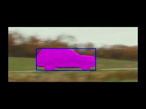
Click to image below to view the video

---

Table of Contents

• Data
• Implementation Guidelines
• Project Structure
• Usage
• Appendix: Disallowed OpenCV Methods

---

Data

• Images:
  A sequence of images is provided in the /data directory, drawn from the VOT 2014 challenge dataset.

• Annotations:

  • groundtruth.txt: Contains bounding boxes for each frame. Each bounding box is given as a comma-separated list of 8 floating-point numbers in (x, y) order representing the four corners (first, second, third, and fourth).

• Augmentations:

  • The detector is trained by extracting feature data from the validation set and then running augmentation algorithms to generate synthetic data to further train the model in a low-data regime manner.

• In-Distribution Test Set:

  • The tracker is successful in detecting vehicles in an in-distribution test set, provided in the data/ directories as movie files.

---

Implementation Details

• Algorithmic Approach

  The vehicle tracker is separated into two components: a detector model and a tracking algorithm.

  The detector is a deep learning model based on a pretrained SegFormer architecture. This architecture generates per-pixel segmentation masks of vehicles. I chose this model because it provides more accurate detection at the pixel level, whereas a model like YOLO-X would only provide bounding boxes. With per-pixel segmentation, detections with partial occlusions—as seen in the sample data (e.g., heavy tree occlusion)—can be precisely trained. It should be acknowledged that segmentation models are not as lightweight or as performant as a bounding-box proposal model; however, the focus of this project is on batch processing of sample data, not necessarily real-time applications.

• Input Features

  • Current RGB pixel data [3 channels, bottom half of input field]
  • Grayscale delta from the previous image in the input sequence [1 channel, top half of input field]
  • Grayscale prior frame data [1 channel, top half of input field]
  • Grayscale current frame data [1 channel, top half of input field]

  The detector model uses the features described above, merging them into one fusion SegFormer model. The additional pixel data beyond the current frame assist with sequence modeling; the model uses prior frame data to better segment the current image by focusing on structural changes rather than just color information.

  The features extracted above worked well. Initially, I tried using only single-frame RGB data, which did not perform significantly well. Then I tried using multiple frames of RGB data, which improved performance by helping the model understand scene changes. I also experimented with incorporating optical flow features, which improved the IoU scoring to 0.94 during validation. However, this approach was slower to train because the OpenCV implementation runs on CPU. As an alternative, the final model used image differencing with grayscale features, which provided similar performance to optical flow but with no additional training overhead.

• Tracker Algorithm

  The tracking algorithm performs object tracking by utilizing the detector model to highlight pixel regions in an image. It proceeds in several phases:

  • Detection Phase:
    As an object moves across the field of view, the detector generates regions, and the tracker associates these detections with objects. The regions are clustered together and assigned to an object using spatial overlap from previous frame data. They can also be clustered by visual similarity and movement vectors to disambiguate overlapping objects.

  • Refinement Phase:
    Once the entire sequence has been processed, a refinement phase is performed. The detection model sometimes over-predicts the boundary of the actual object. The refinement phase runs through all frames of each object’s tracking history and performs a sliding-window refinement process. Cross-correlation scores are used to compare object boundaries between frames and reduce the size of the boundaries to achieve temporal consistency. This step eliminates spurious over-predictions and greatly improves visual tracking stability.

  • Trajectory Generation:
    Object trajectories are generated after the detection and refinement phases. The goal is to create a smooth trajectory based on the object detections from the detection phase. The underlying idea is that vehicles tend to have fixed shapes and, thus, consistent sizes across a sequence of images. The regions are clustered into keyframe groups—sequences where the vehicle maintains a stable visual size. If the visual size becomes unstable (likely due to occlusion or sparse detections), regions with unstable tracking are compared to nearby keyframes, and correspondence matching is performed using cross-correlation to determine how the detected regions map to one another. This mapping helps reconstruct the object’s true size even when detections are partial or missing. After all frames have been assigned correctly positioned and sized regions, a final smoothing pass is performed to finalize the object’s tracking trajectory.

  • Output Visualization:
    Once trajectories are completed, output visualization is performed. If labels are available, a matching algorithm associates labels with objects based on spatial proximity. IoU scoring can then be calculated to determine how well the trajectories perform. Smoothing typically increases the IoU score by a few percentage points. Multiple vehicles can be tracked simultaneously since the tracking algorithm can assign spatially distant regions to different objects; further refinement using visual similarity and other cues can improve the results.

• Training Approach

  PyTorch Lightning was used as the deep learning framework, and the HuggingFace package was used to import models and pre-trained weights. The SegFormer model I chose was pre-trained ImageNet-1k and fine-tuned on CityScapes—a dataset focused on vehicle segmentation. The model consists of approximately 4M parameters, with around 400k in the final decoder module head. This module was adaptively fine-tuned while the rest of the model’s weights were frozen. This strategy keeps the model's early layers focused on vehicle detection without over-fitting to new visual features present in the training set. Surprisingly, the model adaptation worked well with image differencing and gray-scale features, even though these features are out-of-distribution compared to the original training set. The model can be trained in about 5 minutes on a single T4 GPU, within 20–40 epochs depending on the seed.

  The project’s goal was to train a model in a principled manner using only one data sequence, without relying on external data. To achieve this, data augmentation was a significant focus. Initially, the provided sample data was segmented using a Segment Anything model to generate vehicle labels. These labels were reviewed, and poor labels were excluded from training. The final labels consist of extracted vehicle pixels without background, which improves per-pixel detection accuracy. Both the label and background layers are then used for image augmentation during training. The training set is a completely synthetic mixture of random vehicle labels and backgrounds; each image contains one vehicle moving in random directions and positions, with variations in size, color, contrast, hue, rotation, and shearing applied to both background and vehicle pixels. This acts as a form of regularization to help generalize the model and avoid over-fitting.

  The model is trained using various objective functions. A hyperparameter search was performed with different combinations of loss functions. The final combination that worked best was binary cross-entropy (BCE) combined with focal and dice losses, in addition to a total variation loss that acted as a regularizer. This combination helped enforce that detected regions be dense, which is essential for high-quality, confident predictions.

• What Didn’t Work

  • Loss Functions:
    Some loss functions, such as the IoU loss, were unstable and produced poor results. A consistency loss that enforced similarity between the segmentation model's sequence-based outputs acted as too strong a regularizer, causing the model’s training to stagnate (the model could not decide whether to grow or shrink the detected regions, remaining stuck in a local minimum).

  • Single Frame Detection:
    Using only single-frame detection and segmentation did not yield good results. Incorporating multiple frames as input improved performance but led to heavy over-prediction of vehicle boundaries when more frames (up to 5) were used. Optical flow features helped the model understand motion; however, due to their computational cost, image differencing with grayscale features was ultimately used as it provided similar performance without additional training overhead.

  • Occlusion Augmentation:
    Various occlusion augmentation techniques were implemented (e.g., clipping vehicle pixels with stripping and circular patterns). The results were inconclusive because multiple model adjustments were occurring simultaneously, which may have confounded the experiments.

  • Tracker Interpolation:
    Simple smoothing techniques (e.g., sliding-window averages) were not effective in repairing noisy detections. A more targeted approach that focused on refining and filtering the noisy areas of the sequence produced significantly better results, especially for small or distant objects.

• Limitations

  The model has limitations due to its limited training set. It may fail on out-of-distribution data, such as scenes where vehicles are viewed from the front or rear, against urban backgrounds, or with different vehicle types (e.g., trucks). Although the model does detect cars in similar test scenes, synthetic multiple vehicle generation sometimes results in gaps in detection, particularly in regions where the target vehicle has low contrast with the background. The model may overfit to the 'roadway' as a specific detection signal.

  Multiple vehicle tracking is functional but not fully robust. When vehicles overlap, their regions may be clustered together without proper disambiguation, leading to incorrect object assignments as the vehicles move closer together. Visual similarity, speed, and direction of motion could be further leveraged to improve tracking in such cases.

---

Project Structure

A suggested project layout:

vehicle-tracking/
├── README.md
├── requirements.txt           # or environment.yml / poetry.lock
├── src/
│   ├── __init__.py
│   ├── augment_images.py      # helper script used to extract new training/validation data from the sample dataset
│   ├── augment.py             # data augmentation toolkit
│   ├── detector.py            # HuggingFace/PyTorch Lightning framework for model definition and training
│   ├── evaluate.py            # evaluation script for the detector model only
│   ├── loader.py              # PyTorch Dataset/Dataloader definitions
│   ├── losses.py              # Various ML loss/objective functions
│   ├── tracker.py             # main tracking algorithm and evaluation using the detection model
│   └── tools.py               # helper functions, e.g., for data I/O, visualization, mathematical utilities
│   
├── data/
│   ├── groundtruth.txt        # bounding box annotations
│   ├── *.label                # per-frame attribute files
│   ├── *.jpg                  # sample data files used as a validation/evaluation dataset
│   └── *.mp4/*.avi            # sample data files used as in-distribution test set 
│
├── test/
│   ├── __init__.py
│   └── *.py.                  # unit tests and integration tests
│
└── dashboard.py               # StreamLit Dashboard

---

Usage

Installation:
Provide instructions on how to set up your environment. For example:

# Using pip
pip install -r requirements.txt

# or using conda
conda env create -f environment.yml
conda activate vehicle-tracking

Note: It is assumed you have a working CUDA environment for GPU access. If not, the scripts will run using CPU only.

Generate the augmentation data which is required for the sample data tracker. It is best to run this on a GPU enabled system.

python -m src.augment_images

Instead of using the augmented sample data, you can skip this step and run the tracker directly on a data directory. A simple script is provided for convenience.

./run_tracker.sh DATA_DIRECTORY

Training the Detector:

There are prebuilt models already available in the ./checkpoints folder. The detector model can be custom trained using the following command. There currently are no command arguments for this.

python -m src.detector

Running the Tracker:

To run the tracker with the sample data in the ./data/ directory.

python -m src.tracker

The tracker supports various command line options. You can run the following command to see the available options.

python -m src.tracker -h

To run the tracker with all visualization options enabled:

python -m src.tracker --enable_segmentation --enable_smooth_tracking --enable_detection_tracking

For some extra fun, you can add extra synthetic vehicles for additional tracking experiments. This only works with the default dataset, not with custom loaded data.

python -m src.tracker --num_vehicles 4

You can specify a directory for input images. If a groundtruth.txt is available in this directory, it will be used to label the 1st object and produce an IoU score.

python -m src.tracker --dir DATA_DIRECTORY

After the running the tracker, a video output file will be generated with the tracking boxes. You can also review the tracking output in the ./tracking folder. Both can be configured via command line arguments.

Note: When using the default data set, detections are cached to a file. This speeds up tracking generation if there options are changed. To rerun the detections, run the command below. When using custom datasets or other augmentation parameters, the cache file is ignored.

python -m src.tracker --dir DATA_DIRECTORY

By default, only the primary object is tracked. If you have trouble seeing certain vehicle tracking in custom datasets, specify the --detect_all option. This will show all detected objects in the scene.

Dashboard Utility

A StreamLit Dashboard is provided. To run:

streamlit run dashboard.py

Testing:

Tests are almost non-existent. What is provided here is a sample of what more tests could look like.

Run tests with:

PYTHONPATH=. pytest

---

Appendix: Disallowed OpenCV Methods

This project was created with the intention to avoid using the following (and similar) methods as the core of the tracking solution:

• cv::Tracker and its subclasses
• cv::KalmanFilter
• cv::BackgroundSubtractor and its subclasses
• cv::findContours
• cv::matchTemplate
• cv::calcOpticalFlowPyrLK
• cv::calOpticalFlowFarneback
• cv::goodFeaturesToTrack

Note: The code utilized cv::calOpticalFlowFarneback to generate features used to train a detector model as a auxiliary set. However these features are not used during inference. Furthermore, image differencing was just as useful thus optical flow was not necessary for the success of the detector.

---