A Python class for computing Wicksell's transforms of continuous distributions.
Consider a medium consisting in a large number of spheres whose radii follow a Probability Density Function (PDF) f. If sections of the medium are made at random lattitudes, the radius of apparent disks (denoted r below) would follow the PDF [1]:
where E is the mean value of f. The previous formula is refered to as the Wicksell's equation.
The aim of this project is to provide a robust and convinient way to compute the statistics of apparents disks (related to values of r). It is based on histogram decomposition of f, as detailed in [2].
pip install Wicksell
In your Python script, import the class constructor for WicksellTransform:
from Wicksell import wicksell_transform as wt
and create an instance of that class, passing the underlying distribution (that used for computing the Wicksell transform).
transformed_dist = wt.from_continuous(distro)
In the example above, distro must be a continuous distribution, as defined in the scipy's stats module. Finally, use this instance as a usual scipy's distribution. Then all the parameters given to the wt function are actually passed-by and applied to the base-distribution (distro).
In the following, the lognormal distribion is considered.
import scipy.stats as stats
import numpy as np
from Wicksell import wicksell_transform as wt

wlognorm = wt.from_continuous(stats.lognorm)
s = 0.1                 # Shape parameter for lognormal
mu = 0.5
scale = np.exp(mu)  # loc parameter of underlying distribution
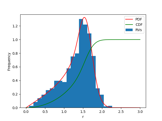
x = np.linspace(0, 3, 1000)
pdf = wlognorm.pdf(x, s, scale=scale)
cdf = wlognorm.cdf(x, s, scale=scale)
data = wlognorm.rvs(s, scale=scale, size=1000, random_state=0)
The random state is fixed here for reproductibility.
from matplotlib import pyplot as plt

fig, ax1 = plt.subplots()
ax1.hist(data, bins=20, density=True, label='RVs')
ax1.set_ylim(bottom=0.0)
ax1.plot(x, pdf, 'r', label='PDF')
ax1.plot(x, cdf, 'g', label='CDF')
ax1.set_ylim(bottom=0.0)
ax1.legend()
ax1.set_xlabel('r')
ax1.set_ylabel('Frequency')
plt.show()
Empirical data can be used to fit the distribution in odrer to get the optimal distribution parameters:
theta = wlognorm.fit(data, floc=0.0)
Here, the fit is made assuming that the location parameter is 0. The fit method is a build-in method provided in all rv_continuous distributions. See the related documentation for details.
The example below roughly leads to:
(0.10258798884347263, 0.0, 1.649539304907202)
It appears that the first parameter is close to s (0.1) whereas the scale (3rd one) corresponds to µ=ln(1.654)=0.5005 (instead of 0.5).
The transformed CDF can be used to perform the Kolmogorov-Smirnov test. For instance, the parameters evaluated by fitting lead to:
stats.kstest(data, wlognorm.cdf, theta)

KstestResult(statistic=0.020989374537414673, pvalue=0.7704283648898784)
Using the histogram decomposition instead of computing the improper integral considerably speeds up the computation of the PDF/CDF. Still, it can be time consuming. Thus the fit method can be slow. Indeed, the example above takes about 100 seconds to complete on an Intel i9 @ 2.30 GHz.
If you use this tool in your research, please cite reference [2].
Feel free to modify and contribute to this software in any manner, as long as your edit complies with the MIT licence. If you have troubles or want to report a bug, please use the issue tracker.
[1] Wicksell, S. D. (1925). The corpuscle problem: A mathematical study of a biometric problem. Biometrika, 17(1/2):84–99, DOI: 10.2307/2332027
[2] Depriester, D. and Kubler, R. (2021). Grain size estimation in polycrystals: solving the corpuscle problem using Maximum Likelihood Estimation. Journal of Structural Geology, 151:104418, ISSN 0191-8141, DOI: 10.1016/j.jsg.2021.104418

