ts2vg: Time series to visibility graphs

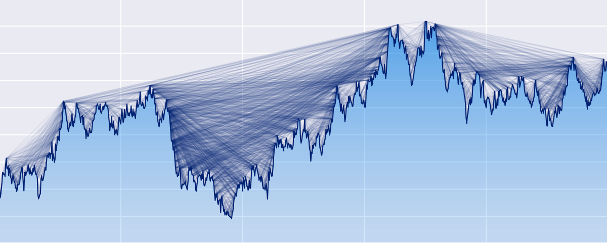
The Python ts2vg package provides high-performance algorithm implementations to build visibility graphs from time series data, as first introduced by Lucas Lacasa et al. in 2008 [1].

The visibility graphs and some of their properties (e.g. degree distributions) are computed quickly and efficiently even for time series with millions of observations. An efficient divide-and-conquer algorithm is used to compute the graphs whenever possible [3].

Installation

The latest released ts2vg version is available at the Python Package Index (PyPI) and can be easily installed by running:

pip install ts2vg

For other advanced uses, to build ts2vg from source Cython is required.

Supported graph types

Main graph types

• Natural Visibility Graphs (NVG) [1] (ts2vg.NaturalVG)
• Horizontal Visibility Graphs (HVG) [2] (ts2vg.HorizontalVG)

Available variations

Additionally, the following variations of the previous main graph types are available:

• Weighted Visibility Graphs (via the weighted parameter)
• Directed Visibility Graphs (via the directed parameter)
• Parametric Visibility Graphs [5] (via the min_weight and max_weight parameters)
• Limited Penetrable Visibility Graphs (LPVG) [4] [6] (via the penetrable_limit parameter)

Note that multiple graph variations can be combined and used at the same time.

Documentation

Usage and reference documentation for ts2vg can be found at carlosbergillos.github.io/ts2vg.

Basic usage

To build a visibility graph from a time series do:

from ts2vg import NaturalVG

ts = [1.0, 0.5, 0.3, 0.7, 1.0, 0.5, 0.3, 0.8]

vg = NaturalVG()
vg.build(ts)

edges = vg.edges

The time series passed (ts) can be any one-dimensional iterable, such as a list or a numpy 1D array.

By default, the input observations are assumed to be equally spaced in time. Alternatively, a second 1D iterable (xs) can be provided for unevenly spaced time series.

Horizontal visibility graphs can be obtained in a very similar way:

from ts2vg import HorizontalVG

ts = [1.0, 0.5, 0.3, 0.7, 1.0, 0.5, 0.3, 0.8]

vg = HorizontalVG()
vg.build(ts)

edges = vg.edges

If we are only interested in the degree distribution of the visibility graph we can pass only_degrees=True to the build method. This will be more efficient in time and memory than storing the whole graph.

vg = NaturalVG()
vg.build(ts, only_degrees=True)

ks, ps = vg.degree_distribution

Directed graphs can be obtained by using the directed parameter and weighted graphs can be obtained by using the weighted parameter:

vg1 = NaturalVG(directed="left_to_right")
vg1.build(ts)

vg2 = NaturalVG(weighted="distance")
vg2.build(ts)

vg3 = NaturalVG(directed="left_to_right", weighted="distance")
vg3.build(ts)

vg4 = HorizontalVG(directed="left_to_right", weighted="h_distance")
vg4.build(ts)

For more information and options see: Examples and API Reference.

Interoperability with other libraries

The graphs obtained can be easily converted to graph objects from other common Python graph libraries such as igraph, NetworkX and SNAP for further analysis.

The following methods are provided:

• as_igraph()
• as_networkx()
• as_snap()

For example:

vg = NaturalVG()
vg.build(ts)

g = vg.as_networkx()

Command line interface

ts2vg can also be used as a command line program directly from the console:

ts2vg ./timeseries.txt -o out.edg

For more help and a list of options run:

ts2vg --help

Contributing

ts2vg can be found on GitHub. Pull requests and issue reports are welcome.

License

ts2vg is licensed under the terms of the MIT License.

References

[1]	(1, 2) Lucas Lacasa et al., "From time series to complex networks: The visibility graph", 2008.

[2]	Lucas Lacasa et al., "Horizontal visibility graphs: exact results for random time series", 2009.

[3]	Xin Lan et al., "Fast transformation from time series to visibility graphs", 2015.

[4]	T.T Zhou et al., "Limited penetrable visibility graph for establishing complex network from time series", 2012.

[5]	I.V. Bezsudnov et al., "From the time series to the complex networks: The parametric natural visibility graph", 2014

[6]	Qi Xuan et al., "CLPVG: Circular limited penetrable visibility graph as a new network model for time series", 2021