There are many deep learning libraries, each with its own approach. What are the advantages and drawbacks of each library, in terms of system optimization and user experience? This topic compares the programming models, discusses the fundamental advantages and drawbacks of each, and explores how we can learn from them.
We don't benchmark deep learning libraries in this topic. We focus on the programming models themselves, instead of the implementation. We divide the libraries into several categories by the type of user interface, and discuss how interface style affects the performance and flexibility. The discussion isn't specific to deep learning, but we use deep learning applications for our use cases and optimization as our goal.
Let's compare symbolic-style programs with imperative-style programs. If you are a Python or C++ programmer, you're already familiar with imperative programs. Imperative-style programs perform computation as you run them. Most code you write in Python is imperative, as is the following NumPy snippet.
    import numpy as np
    a = np.ones(10)
    b = np.ones(10) * 2
    c = b * a
    d = c + 1
When the program executes c = b * a, it runs the actual computation.
Symbolic programs are a bit different.
The following snippet is an equivalent symbolic-style program that achieves the same goal of calculating d.
    A = Variable('A')
    B = Variable('B')
    C = B * A
    D = C + Constant(1)
    # compiles the function
    f = compile(D)
    d = f(A=np.ones(10), B=np.ones(10)*2)
The difference in symbolic programs is that when C = B * A is executed, no computation occurs.
Instead, these operations generate a computation graph (symbolic graph) that represents the computation.
The following figure shows a computation graph to compute D.
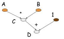
Most symbolic-style programs contain, either explicitly or implicitly, a compile step. This converts the computation graph into a function that can be called. Computation occurs in the last step in the code. The major characteristic of symbolic programs is the clear separation between defining the computation graph and compiling.
Examples of imperative-style deep learning libraries include Torch, Chainer, and Minerva. Examples of symbolic-style deep learning libraries include Theano, CGT, and TensorFlow. Libraries that use configuration files, like CXXNet and Caffe, can also be viewed as symbolic-style libraries, where the content in the configuration file defines the computation graph.
Now that you understand the difference between the two programming models, let's compare them.
This is a general statement that might not be strictly true, but imperative programs are usually more flexible than symbolic programs. When you're writing an imperative-style program in Python, you are writing in Python. When you're writing a symbolic program, it's different. Consider the following imperative program, and think about how you can translate this into a symbolic program.
    a = 2
    b = a + 1
    d = np.zeros(10)
    for i in range(d):
        d += np.zeros(10)
It's not easy, because there's a Python for-loop that might not be readily supported by the symbolic API. When you write a symbolic program in Python, you're not writing in Python. Instead, you're writing a domain-specific language (DSL) defined by the symbolic API. The symbolic APIs are more powerful versions of DSL that generate the computation graphs or the configuration of neural networks. In that sense, config-file input libraries are all symbolic.
Because imperative programs are more native than symbolic programs, it's easier to use native language features--such as printing out the values in the middle of computation and using conditioning and loops in the host language--and inject them into the computation flow.
As we've seen, imperative programs are usually more flexible and native to the host language. Then why are more deep learning libraries symbolic? The main reason is efficiency, both in terms of memory and runtime. Let's consider the same example we used in the beginning of this section.
    import numpy as np
    a = np.ones(10)
    b = np.ones(10) * 2
    c = b * a
    d = c + 1
    ...
Assume that each cell in the array costs 8 bytes. How much memory do you need to execute this program in the Python console?
You need memory for 4 arrays of size 10, that means you need 4 * 10 * 8 = 320 bytes. On the other hand,
to execute the computation graph, you can reuse the memory of C and D, to do the last computation in-place. This requires just 3 * 10 * 8 = 240
bytes.
Symbolic programs are more restricted. When you call compile on D, you tell the system that only the value of
D is needed. The intermediate values of the computation, in this case C, are invisible to you.
This allows symbolic programs to safely reuse the memory for in-place computation.
On the other hand, imperative programs need to be prepared to encounter all possible demands. If you run the preceding program in a Python console, it's possible that any of the variables could be used in the future. This prevents the system from sharing variable memory space.
Of course, this is somewhat misleading, because garbage collection can occur in imperative programs and memory could then be reused. However, imperative programs do need to be "prepared to encounter all possible demands," and this limits the optimization you can perform. This is true for non-trivial cases, such as gradient calculation, which we discuss in next section.
Symbolic programs can perform another kind of optimization, operation folding. In the example programs, the multiplication and addition operations can be folded into one operation, as shown in the following graph. If the computation runs on a GPU processor, one GPU kernel will be executed, instead of two. This is what we do to hand-crafted operations in optimized libraries, such as CXXNet and Caffe. Operation folding improves computation efficiency.
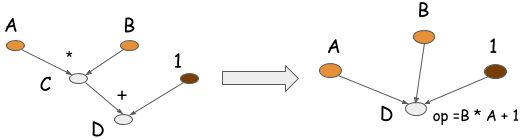
You can't perform operation folding in imperative programs, because the intermediate value might be referenced in the future. Operation folding is possible in symbolic programs because you get the entire computation graph, and a clear boundary on which value is needed and which isn't. Imperative programs operate only on local operations and do not have such a clear boundary.
In this section, we compare how the two programming models perform on the problem of auto differentiation, or backpropagation. All deep learning libraries need to solve the problem of gradient calculation. Both imperative and symbolic programs can perform gradient calculation.
Let's start with imperative programs. The following example Python code performs automatic differentiation in the example we've used in this topic.
    class array(object) :
        """Simple Array object that support autodiff."""
        def __init__(self, value, name=None):
            self.value = value
            if name:
                self.grad = lambda g : {name : g}

        def __add__(self, other):
            assert isinstance(other, int)
            ret = array(self.value + other)
            ret.grad = lambda g : self.grad(g)
            return ret

        def __mul__(self, other):
            assert isinstance(other, array)
            ret = array(self.value * other.value)
            def grad(g):
                x = self.grad(g * other.value)
                x.update(other.grad(g * self.value))
                return x
            ret.grad = grad
            return ret

    # some examples
    a = array(1, 'a')
    b = array(2, 'b')
    c = b * a
    d = c + 1
    print d.value
    print d.grad(1)
    # Results
    # 3
    # {'a': 2, 'b': 1}
In this code, each array object contains a grad function (it is actually a closure).
When you run d.grad, it recursively invokes the grad function of its inputs, backprops the gradient value back, and
returns the gradient value of each input.
This might look a bit complicated, so let's consider the gradient calculation for symbolic programs. The following program performs symbolic gradient calculation for the same task.
    A = Variable('A')
    B = Variable('B')
    C = B * A
    D = C + Constant(1)
    # get gradient node.
    gA, gB = D.grad(wrt=[A, B])
    # compiles the gradient function.
    f = compile([gA, gB])
    grad_a, grad_b = f(A=np.ones(10), B=np.ones(10)*2)
The grad function of D generates a backward computation graph, and returns a gradient node, gA, gB, which
correspond to the red nodes in the following figure.
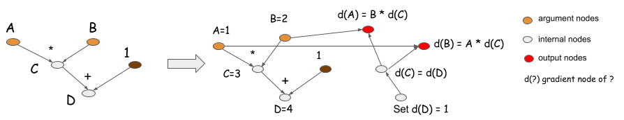
The imperative program actually does the same thing as the symbolic program. It implicitly saves a backward
computation graph in the grad closure. When you invoked d.grad, you start from d(D),
backtrack the graph to compute the gradient, and collect the results back.
The gradient calculation in both symbolic and imperative programming follows the same
pattern. What's the difference then? Recall the be prepared to encounter all possible demands
the requirement of imperative programs. If you are creating an array library that supports automatic differentiation,
you have to keep the grad closure along with the computation. This means that none of the history variables can be
garbage collected because they are referenced by variable d by way of function closure.
What if you want to compute only the value of d, and don't want the gradient value? In symbolic programming, you declare this with f=compiled([D]). This also declares the boundary
of computation, telling the system that you want to compute only the forward pass. As a result, the system can
free the memory of previous results, and share the memory between inputs and outputs.
Imagine running a deep neural network with n layers.
If you are running only the forward pass, not the backward(gradient) pass, you need to allocate only two copies of
temporal space to store the values of the intermediate layers, instead of n copies of them.
However, because imperative programs need to be prepared to encounter all possible demands of getting the gradient,
they have to store the intermediate values, which requires n copies of temporal space.
As you can see, the level of optimization depends on the restrictions on what you can do. Symbolic programs ask you to clearly specify the boundary of computation by compiling or its equivalent. Imperative programs prepare to encounter all possible demands. Symbolic programs have a natural advantage because they know more about what you do and don't want.
Of course, you can also enhance imperative programs to impose restrictions. For example, one solution to the preceding problem is to introduce a context variable. You can introduce a no gradient context variable to turn gradient calculation off. This provides an imperative program with the ability to impose some restrictions, but reduces efficiency.
    with context.NoGradient():
        a = array(1, 'a')
        b = array(2, 'b')
        c = b * a
        d = c + 1
However, this example still must be prepared to encounter all possible demands, which means that you can't perform the in-place calculation to reuse the memory in the forward pass (a trick commonly used to reduce GPU memory usage). The techniques we've discussed generate an explicit backward pass. Some of the libraries such as Caffe and CXXNet perform backprop implicitly on the same graph. The approach we've discussed in this section also applies to them.
Most configuration-file-based libraries, such as CXXNet and Caffe are designed to meet one or two generic requirements: get the activation of each layer, or get the gradient of all of the weights. These libraries have the same problem: the more generic operations the library has to support, the less optimization (memory sharing) you can do, based on the same data structure.
As you can see, the trade-off between restriction and flexibility is the same for most cases.
It's important to able to save a model and load it back later. There are different ways to save your work. Normally, to save a neural network, you need to save two things: a net configuration for the structure of the neural network and the weights of the neural network.
The ability to check the configuration is a plus for symbolic programs. Because the symbolic construction phase does perform computation, you can directly serialize the computation graph, and load it back later. This solves the problem of saving the configuration without introducing an additional layer.
    A = Variable('A')
    B = Variable('B')
    C = B * A
    D = C + Constant(1)
    D.save('mygraph')
    ...
    D2 = load('mygraph')
    f = compile([D2])
    # more operations
    ...
Because an imperative program executes as it describes the computation, you have to save the code itself as the configuration, or build another
configuration layer on top of the imperative language.
Most symbolic programs are data flow (computation) graphs. Data flow graphs describe computation. but it's is not obvious how to use graphs to describe parameter updates. That's because parameter updates introduce mutation, which is not a data flow concept. Most symbolic programs introduce a special update statement to update some persistent states of the programs.
It's usually easier to write parameter updates in imperative style, especially when you need multiple updates that relate to each other. For symbolic programs, the update statement is also executed as you call it. So in that sense, most symbolic deep learning libraries fall back on the imperative approach to perform updates, while using the symbolic approach to perform gradient calculation.
In comparing the two programming styles, some of our arguments might not be strictly true. However, most of the principles hold true in general, and apply when creating deep learning libraries. We've concluded that there is no clear boundary between programming styles. For example, you can create a just-in-time (JIT) compiler in Python to compile imperative Python programs, which provides some of the advantages of global information held in symbolic programs.
Let's talk about the operations supported by deep learning libraries. Usually, there are two types of operations supported by various deep learning libraries:
- Big layer operations, such as FullyConnected and BatchNormalize
- Small operations, such as element-wise addition and multiplication
Libraries like CXXNet and Caffe support layer-level operations. Libraries like Theano and Minerva support fine-grained operations.
It's quite natural to use smaller operations to compose bigger operations. For example, the sigmoid unit can be simply be composed of division and an exponential:
sigmoid(x) = 1.0 / (1.0 + exp(-x))Using smaller operations as building blocks, you can express most of the problems you want. If you're more familiar with CXXNet- or Caffe-style layers, note that these operations don't differ from a layer, except that they are smaller.
SigmoidLayer(x) = EWiseDivisionLayer(1.0, AddScalarLayer(ExpLayer(-x), 1.0))This expression composes three layers, with each defining its forward and backward (gradient) function. Using smaller operations gives you the advantage of building new layers quickly, because you only need to compose the components.
Directly composing sigmoid layers requires three layers of operation, instead of one.
SigmoidLayer(x) = EWiseDivisionLayer(1.0, AddScalarLayer(ExpLayer(-x), 1.0))This code creates overhead for computation and memory (which could be optimized, with cost).
Libraries like CXXNet and Caffe take a different approach. To support coarse-grained operations, such as BatchNormalization and the SigmoidLayer directly, in each layer, the calculation kernel is hand crafted with one or only some CUDA kernel launches. This makes these implementations more efficient.
Can small operations be optimized? Of course, they can. Let's look at the system optimization part of the compilation engine. Two types of optimization can be performed on the computation graph:
- Memory allocation optimization, to reuse the memory of the intermediate computations.
- Operator fusion, to detect sub-graph patterns, such as the sigmoid, and fuse them into a bigger operation kernel.
Memory allocation optimization isn't restricted to small operations graphs. You can use it with bigger operations graph, too. However, optimization might not be essential for bigger operation libraries like CXXNet and Caffe, because you can't find the compilation step in them. However, there's a (dumb) compilation step in these libraries, that basically translates the layers into a fixed forward, backprop execution plan, by running each operation one by one.
For computation graphs with smaller operations, these optimizations are crucial to performance. Because the operations are small, there are many sub-graph patterns that can be matched. Also, because the final generated operations might not be able to be enumerated, an explicit recompilation of the kernels is required, as opposed to the fixed amount of precompiled kernels in the big operation libraries. This creates compilation overhead for the symbolic libraries that support small operations. Requiring compilation optimization also creates engineering overhead for the libraries that solely support smaller operations.
As in the case of symbolic vs imperative, the bigger operation libraries "cheat" by asking you to provide restrictions (to the common layer), so that you actually perform the sub-graph matching. This moves the compilation overhead to the real brain, which is usually not too bad.
You always have a need to write small operations and compose them. Libraries like Caffe use hand-crafted kernels to build these bigger blocks. Otherwise, you would have to compose smaller operations using Python.
There's a third choice that works pretty well. This is called the expression template. Basically, you use template programming to generate generic kernels from an expression tree at compile time. For details, see Expression Template Tutorial. CXXNet makes extensive use of an expression template, which enables creating much shorter and more readable code that matches the performance of hand-crafted kernels.
The difference between using an expression template and Python kernel generation is that expression evaluation is done at compile time for C++ with an existing type, so there is no additional runtime overhead. In principle, this is also possible with other statically typed languages that support templates, but we've seen this trick used only in C++.
Expression template libraries create a middle ground between Python operations and hand-crafted big kernels by allowing C++ users to craft efficient big operations by composing smaller operations. It's an option worth considering.
Now that we've compared the programming models, which should you choose? Before delving into that, we should emphasize that depending on the problems you're trying to solve, our comparison mighty not necessarily have a big impact.
Remember Amdahl's law: If you are optimizing a non-performance-critical part of your problem, you won't get much of a performance gain.
As you've seen, there usually is a trade-off between efficiency, flexibility, and engineering complexity. The more suitable programming style depends on the problem you are trying to solve. For example, imperative programs are better for parameter updates, and symbolic programs for gradient calculation.
We advocate mixing the approaches. Recall Amdahl's law. Sometimes the part that we want to be flexible isn't necessarily crucial to performance. It's okay to be a bit sloppy to support more flexible interfaces. In machine learning, combining methods usually works better than using just one.
If you can combine the programming models correctly, you can get better results than you can use a single programming model. In this section, we discuss how to do so.
There are two ways to mix symbolic and imperative programs:
- Use imperative programs within symbolic programs as callbacks
- Use symbolic programs as part of imperative programs
We've observed that it's usually helpful to write parameter updates imperatively, and perform gradient calculations in symbolic programs.
Symbolic libraries already mix programs because Python itself is imperative. For example, the following program mixes the symbolic approach with NumPy, which is imperative.
    A = Variable('A')
    B = Variable('B')
    C = B * A
    D = C + Constant(1)
    # compiles the function
    f = compile(D)
    d = f(A=np.ones(10), B=np.ones(10)*2)
    d = d + 1.0
The symbolic graphs are compiled into a function that can be executed imperatively. The internals are a black box to the user. This is exactly like writing C++ programs and exposing them to Python, which we commonly do.
Because parameter memory resides on the GPU, you might not want to use NumPy as an imperative component. Supporting a GPU-compatible imperative library that interacts with symbolic compiled functions or provides a limited amount of updating syntax in the update statement in symbolic program execution might be a better choice.
There might be a good reason to combine small and big operations. Consider applications that perform tasks such as changing a loss function or adding a few customized layers to an existing structure. Usually, you can use big operations to compose existing components, and use smaller operations to build the new parts.
Recall Amdahl's law. Often, the new components might not be the cause of the computation bottleneck. Because the performance-critical part is already optimized by the bigger operations, it's okay to forego optimizing the additional small operations, or to do a limited amount of memory optimization instead of operation fusion and directly running them.
The goal of this topic is to compare the approaches of deep learning programs. We've found that there might not be a universal solution, but that you can choose your approach, or combine the approaches that you like to create more interesting and intelligent deep learning libraries.
This topic is part of our effort to provide open-source system design notes for deep learning libraries. We welcome your contributions.