Raphael Gottardo
December 8, 2014
Let's first turn on the cache for increased performance.
# Set some global knitr options
library("knitr")
opts_chunk$set(tidy=TRUE, tidy.opts=list(blank=FALSE, width.cutoff=80), cache=TRUE)-
R has pass-by-value semantics, which minimizes accidental side effects. However, this can become a major bottleneck when dealing with large datasets both in terms of memory and speed.
-
Working with
data.frames in R can also be painful process in terms of writing code. -
Fortunately, R provides some solution to this problems.
Here we will review three R packages that can be used to provide efficient data manipulation:
data.table: An package for efficient data storage and manipulationRSQLite: Database Interface R driver for SQLitesqldf: An R package for runing SQL statements on R data frames, optimized for convenience
Thank to Kevin Ushey (@kevin_ushey) for the data.table notes and Matt Dowle and Arunkumar Srinivasan for helpful comments.
data.table is an R package that extends. R data.frames.
Under the hood, they are just `data.frame's, with some extra 'stuff' added on. So, they're collections of equal-length vectors. Each vector can be of different type.
library(data.table)
dt <- data.table(x = 1:3, y = c(4, 5, 6), z = letters[1:3])
dt
## x y z
## 1: 1 4 a
## 2: 2 5 b
## 3: 3 6 c
class(dt)## [1] "data.table" "data.frame"
The extra functionality offered by data.table allows us to modify, reshape, and merge data.tables much quicker than data.frames. See that data.table inherits from data.frame!
- stable CRAN release
# Only install if not already installed.
require(data.table) || install.packages("data.table")- latest bug-fixes + enhancements (No need to do that, we will use the stable release)
library(devtools)
install_github("Rdatatable/data.table", build_vignettes = FALSE)Most of your interactions with data.tables will be through the subset ([)
operator, which behaves quite differently for data.tables. We'll examine
a few of the common cases.
Visit this stackoverflow question for a summary of the differences between data.frames and data.tables.
library(data.table)
DF <- data.frame(x = 1:3, y = 4:6, z = 7:9)
DT <- data.table(x = 1:3, y = 4:6, z = 7:9)
DF[c(2, 3)]
## y z
## 1 4 7
## 2 5 8
## 3 6 9
DT[c(2, 3)]## x y z
## 1: 2 5 8
## 2: 3 6 9
By default, single-element subsetting in data.tables refers to rows, rather
than columns.
library(data.table)
DF <- data.frame(x = 1:3, y = 4:6, z = 7:9)
DT <- data.table(x = 1:3, y = 4:6, z = 7:9)
DF[c(2, 3), ]
## x y z
## 2 2 5 8
## 3 3 6 9
DT[c(2, 3), ]## x y z
## 1: 2 5 8
## 2: 3 6 9
Notice: row names are lost with data.tables. Otherwise, output is identical.
library(data.table)
DF <- data.frame(x = 1:3, y = 4:6, z = 7:9)
DT <- data.table(x = 1:3, y = 4:6, z = 7:9)
DF[, c(2, 3)]
## y z
## 1 4 7
## 2 5 8
## 3 6 9
DT[, c(2, 3)]## [1] 2 3
DT[, c(2,3)] just returns c(2, 3). Why on earth is that?
The subset operator is really a function, and data.table modifies it to behave
differently.
Call the arguments we pass e.g. DT[i, j], or DT[i].
The second argument to [ is called the j expression, so-called because it's
interpreted as an R expression. This is where most of the data.table
magic happens.
j is an expression evaluated within the frame of the data.table, so
it sees the column names of DT. Similarly for i.
First, let's remind ourselves what an R expression is.
An expression is a collection of statements, enclosed in a block generated by
braces {}.
## an expression with two statements
{
    x <- 1
    y <- 2
}
## the last statement in an expression is returned
k <- {
    print(10)
    5
}
## [1] 10
print(k)## [1] 5
So, data.table does something special with the expression that you pass as
j, the second argument, to the subsetting ([) operator.
The return type of the final statement in our expression determines the type of operation that will be performed.
In general, the output should either be a list of symbols, or a statement
using :=.
We'll start by looking at the list of symbols as an output.
When we simply provide a list to the j expression, we generate a new
data.table as output, with operations as performed within the list call.
library(data.table)
DT <- data.table(x = 1:5, y = 1:5)
DT[, list(mean_x = mean(x), sum_y = sum(y), sumsq = sum(x^2 + y^2))]
## mean_x sum_y sumsq
## 1: 3 15 110
Notice how the symbols x and y are looked up within the data.table DT.
No more writing DT$ everywhere!
Using the := operator tells us we should assign columns by reference into
the data.table DT:
library(data.table)
DT <- data.table(x = 1:5)
DT[, `:=`(y, x^2)]
## x y
## 1: 1 1
## 2: 2 4
## 3: 3 9
## 4: 4 16
## 5: 5 25
By default, data.tables are not copied on a direct assignment <-:
library(data.table)
DT <- data.table(x = 1)
DT2 <- DT
DT[, `:=`(y, 2)]
## x y
## 1: 1 2
DT2## x y
## 1: 1 2
Notice that DT2 has changed. This is something to be mindful of; if you want
to explicitly copy a data.table do so with DT2 <- copy(DT).
library(data.table)
DT <- data.table(x = 1:5, y = 6:10, z = 11:15)
DT[, `:=`(m, log2((x + 1)/(y + 1)))]
## x y z m
## 1: 1 6 11 -1.8073549
## 2: 2 7 12 -1.4150375
## 3: 3 8 13 -1.1699250
## 4: 4 9 14 -1.0000000
## 5: 5 10 15 -0.8744691
Note that the right-hand side of a := call can be an expression.
library(data.table)
DT <- data.table(x = 1:5, y = 6:10, z = 11:15)
DT[, `:=`(m, {
    tmp <- (x + 1)/(y + 1)
    log2(tmp)
})]
## x y z m
## 1: 1 6 11 -1.8073549
## 2: 2 7 12 -1.4150375
## 3: 3 8 13 -1.1699250
## 4: 4 9 14 -1.0000000
## 5: 5 10 15 -0.8744691
The left hand side of a := call can also be a character vector of names,
for which the corresponding final statement in the j expression should be
a list of the same length.
library(data.table)
DT <- data.table(x = 1:5, y = 6:10, z = 11:15)
DT[, `:=`(c("m", "n"), {
    tmp <- (x + 1)/(y + 1)
    list(log2(tmp), log10(tmp))
})]
## x y z m n
## 1: 1 6 11 -1.8073549 -0.5440680
## 2: 2 7 12 -1.4150375 -0.4259687
## 3: 3 8 13 -1.1699250 -0.3521825
## 4: 4 9 14 -1.0000000 -0.3010300
## 5: 5 10 15 -0.8744691 -0.2632414
DT[, `:=`(a = x^2, b = y^2)]## x y z m n a b
## 1: 1 6 11 -1.8073549 -0.5440680 1 36
## 2: 2 7 12 -1.4150375 -0.4259687 4 49
## 3: 3 8 13 -1.1699250 -0.3521825 9 64
## 4: 4 9 14 -1.0000000 -0.3010300 16 81
## 5: 5 10 15 -0.8744691 -0.2632414 25 100
DT[, `:=`(c("c", "d"), list(x^2, y^2))]## x y z m n a b c d
## 1: 1 6 11 -1.8073549 -0.5440680 1 36 1 36
## 2: 2 7 12 -1.4150375 -0.4259687 4 49 4 49
## 3: 3 8 13 -1.1699250 -0.3521825 9 64 9 64
## 4: 4 9 14 -1.0000000 -0.3010300 16 81 16 81
## 5: 5 10 15 -0.8744691 -0.2632414 25 100 25 100
So, we typically call j the j expression, but really, it's either:
-
An expression, or
-
A call to the function
:=, for which the first argument is a set of names (vectors to update), and the second argument is an expression, with the final statement typically being a list of results to assign within thedata.table.
As I said before, a := b is parsed by R as ":="(a, b), hence it
looking somewhat like an operator.
quote(`:=`(a, b))## `:=`(a, b)
Whenever you sub-assign a data.frame, R is forced to copy the entire
data.frame.
That is, whenever you write DF$x <- 1, DF["x"] <- 1, DF[["x"]] <- 1...
... R will make a copy of DF before assignment.
This is done in order to ensure any other symbols pointing at the same object
do not get modified. This is a good thing for when we need to reason about
the code we write, since, in general, we expect R to operate without side
effects.
Unfortunately, it is prohibitively slow for large objects, and hence why
:= can be very useful.
library(data.table)
library(microbenchmark)
big_df <- data.frame(x = rnorm(1e+06), y = sample(letters, 1e+06, TRUE))
big_dt <- data.table(big_df)
microbenchmark(big_df$z <- 1, big_dt[, `:=`(z, 1)])
## Unit: milliseconds
## expr min lq mean median uq max
## big_df$z <- 1 1.325358 2.331905 5.860944 2.544618 4.37489 105.6464
## big_dt[, `:=`(z, 1)] 2.536554 4.295727 8.677173 5.066026 7.62658 128.0590
## neval cld
## 100 a
## 100 a
Once again, notice that := is actually a function, and z := 1
is parsed as ":="(z, 1).
We can also perform grouping like operations through the use of the
by argument:
library(data.table)
DT <- data.table(x = 1:5, y = 6:10, gp = c("a", "a", "a", "b", "b"))
DT[, `:=`(z, mean(x + y)), by = gp]
## x y gp z
## 1: 1 6 a 9
## 2: 2 7 a 9
## 3: 3 8 a 9
## 4: 4 9 b 14
## 5: 5 10 b 14
Notice that since mean(x+y) returns a scalar (numeric vector of length 1), it is recycled to fill within each group.
What if, rather than modifying the current data.table, we wanted to generate
a new one?
library(data.table)
DT <- data.table(x = 1:5, y = 6:10, gp = c("a", "a", "a", "b", "b"))
DT[, list(z = mean(x + y)), by = gp]
## gp z
## 1: a 9
## 2: b 14
Notice that we retain one row for each unique group specified in the by
argument, and only the by variables along-side our z variable are returned.
- A
list
... returns a new data.table, potentially subset over groups in your by.
- A
:=Call
... modifies that data.table in place, hence saving memory. Output is
recycled if the by argument is used.
-
an expression, with the final (or only) statement being a
listof (named) arguments, -
a call to the
:=function, with
- the first argument being names, and
- the second argument being an expression, for which the last statement is a list of the same length as the first argument.
There are a number of special variables defined only within j, that allow us to do some neat things...
library(data.table)
data.table()[, ls(all = TRUE)]
## [1] ".GRP" ".I" ".N" ".SD"
These variables allow us to infer a bit more about what's going on within the
data.table calls, and also allow us to write more complicated j expressions.
A data.table containing the subset of data for each group, excluding
columns used in by.
A list containing a length 1 vector for each item in by.
An integer, length 1, containing the number of rows in .SD.
A vector of indices, holding the row locations from which .SD was
pulled from the parent DT.
A counter telling you which group you're working with (1st, 2nd, 3rd...)
Compute the counts, by group, using data.table...
set.seed(123)
library(data.table)
library(microbenchmark)
DT <- data.table(x = sample(letters[1:3], 1e+05, TRUE))
DT[, .N, by = x]
## x N
## 1: a 33387
## 2: c 33201
## 3: b 33412
table(DT$x)##
## a b c
## 33387 33412 33201
library(data.table)
library(microbenchmark)
DT <- data.table(x = factor(sample(letters[1:3], 1e+05, TRUE)))
microbenchmark(tbl = table(DT$x), DT = DT[, .N, by = x])
## Unit: milliseconds
## expr min lq mean median uq max neval cld
## tbl 8.535709 10.253819 12.447354 11.502042 13.22827 25.109841 100 b
## DT 1.112893 1.403274 1.780877 1.590881 1.90645 4.514918 100 a
library(data.table)
DT <- data.table(x = rnorm(10), y = rnorm(10), z = rnorm(10), id = letters[1:10])
DT[, lapply(.SD, mean), .SDcols = c("x", "y", "z")]
## x y z
## 1: -0.2511676 0.7089166 0.4615515
lapply(DT[, 1:3, with = FALSE], mean)## $x
## [1] -0.2511676
##
## $y
## [1] 0.7089166
##
## $z
## [1] 0.4615515
library(data.table)
library(microbenchmark)
DT <- data.table(x = rnorm(1e+05), y = rnorm(1e+05), z = sample(letters, 1e+05, replace = TRUE))
DT2 <- copy(DT)
setkey(DT2, "z")
microbenchmark(DT = DT[, lapply(.SD, mean), .SDcols = c("x", "y"), by = "z"], DT2 = DT2[,
    lapply(.SD, mean), .SDcols = c("x", "y"), by = "z"])
## Unit: milliseconds
## expr min lq mean median uq max neval cld
## DT 2.013897 2.485728 2.99011 2.684291 3.390388 5.935036 100 b
## DT2 1.995405 2.235107 2.69206 2.397125 2.779748 9.285968 100 a
setting a key can lead to faster grouping operations.
data.tables can be keyed, allowing for faster indexing and subsetting. Keys
are also used for joins, as we'll see later.
library(data.table)
DT <- data.table(x = c("a", "a", "b", "c", "a"), y = rnorm(5))
setkey(DT, x)
DT["a"]  ## grabs rows corresponding to 'a'
## x y
## 1: a 1.3242525
## 2: a 3.2439986
## 3: a 0.6207716
Note that this does a binary search rather than a vector scan, which is
much faster!
library(data.table)
library(microbenchmark)
DF <- data.frame(key = sample(letters, 1e+06, TRUE), x = rnorm(1e+06))
DT <- data.table(DF)
setkey(DT, key)
identical(DT["a"]$x, DF[DF$key == "a", ]$x)
## [1] TRUE
microbenchmark(DT = DT["a"], DF = DF[DF$key == "a", ], times = 5)## Unit: milliseconds
## expr min lq mean median uq max
## DT 3.009992 3.641566 3.88202 3.762855 3.949109 5.046576
## DF 160.408577 189.953657 199.53043 202.004269 202.728430 242.557198
## neval cld
## 5 a
## 5 b
Further reading: you can set multiple keys with setkeyv as well.
data.table comes with many kinds of joins, implements through the
merge.data.table function, and also through the [ syntax as well. We'll
focus on using merge.
library(data.table)
library(microbenchmark)
DT1 <- data.table(x = c("a", "a", "b", "dt1"), y = 1:4)
DT2 <- data.table(x = c("a", "b", "dt2"), z = 5:7)
setkey(DT1, x)
setkey(DT2, x)
merge(DT1, DT2)
## x y z
## 1: a 1 5
## 2: a 2 5
## 3: b 3 6
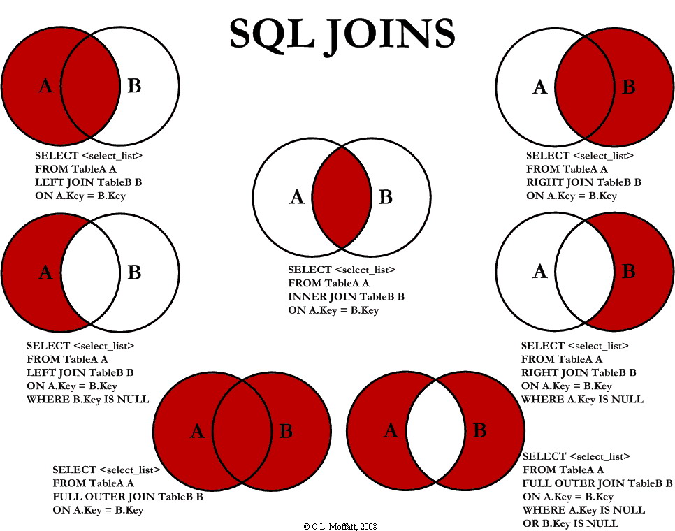
Here is a quick summary of SQL joins, applicable to data.table too.
(Source: http://www.codeproject.com)
library(data.table)
library(microbenchmark)
DT1 <- data.table(x = c("a", "a", "b", "dt1"), y = 1:4)
DT2 <- data.table(x = c("a", "b", "dt2"), z = 5:7)
setkey(DT1, x)
setkey(DT2, x)
merge(DT1, DT2, all.x = TRUE)
## x y z
## 1: a 1 5
## 2: a 2 5
## 3: b 3 6
## 4: dt1 4 NA
library(data.table)
library(microbenchmark)
DT1 <- data.table(x = c("a", "a", "b", "dt1"), y = 1:4)
DT2 <- data.table(x = c("a", "b", "dt2"), z = 5:7)
setkey(DT1, x)
setkey(DT2, x)
merge(DT1, DT2, all.y = TRUE)
## x y z
## 1: a 1 5
## 2: a 2 5
## 3: b 3 6
## 4: dt2 NA 7
library(data.table)
library(microbenchmark)
DT1 <- data.table(x = c("a", "a", "b", "dt1"), y = 1:4)
DT2 <- data.table(x = c("a", "b", "dt2"), z = 5:7)
setkey(DT1, x)
setkey(DT2, x)
merge(DT1, DT2, all = TRUE)  ## outer join
## x y z
## 1: a 1 5
## 2: a 2 5
## 3: b 3 6
## 4: dt1 4 NA
## 5: dt2 NA 7
library(data.table)
library(microbenchmark)
DT1 <- data.table(x = c("a", "a", "b", "dt1"), y = 1:4)
DT2 <- data.table(x = c("a", "b", "dt2"), z = 5:7)
setkey(DT1, x)
setkey(DT2, x)
merge(DT1, DT2, all = FALSE)  ## inner join
## x y z
## 1: a 1 5
## 2: a 2 5
## 3: b 3 6
library(data.table)
library(microbenchmark)
DT1 <- data.table(x = do.call(paste, expand.grid(letters, letters, letters, letters)),
    y = rnorm(26^4))
DT2 <- DT1[sample(1:nrow(DT1), 1e+05), ]
setnames(DT2, c("x", "z"))
DF1 <- as.data.frame(DT1)
DF2 <- as.data.frame(DT2)
setkey(DT1, x)
setkey(DT2, x)
microbenchmark(DT = merge(DT1, DT2), DF = merge.data.frame(DF1, DF2), replications = 5)
## Unit: nanoseconds
## expr min lq mean median uq
## DT 43588481 47473113.5 5.960710e+07 50444820 60420617.5
## DF 864700111 947929331.0 1.068524e+09 997906140 1170151161.5
## replications 6 38.5 1.876600e+02 174 245.5
## max neval cld
## 166500058 100 b
## 1944960095 100 c
## 651 100 a
We can also perform joins of two keyed data.tables using the [ operator.
We perform right joins, so that e.g.
DT1[DT2]
is a right join of DT1 into DT2. These joins are typically a bit faster. Do
note that the order of columns post-merge can be different, though.
library(data.table)
library(microbenchmark)
DT1 <- data.table(x = do.call(paste, expand.grid(letters, letters, letters, letters)),
    y = rnorm(26^4))
DT2 <- DT1[sample(1:nrow(DT1), 1e+05), ]
setnames(DT2, c("x", "z"))
setkey(DT1, x)
setkey(DT2, x)
tmp1 <- DT2[DT1]
setcolorder(tmp1, c("x", "y", "z"))
tmp2 <- merge(DT1, DT2, all.x = TRUE)
setcolorder(tmp2, c("x", "y", "z"))
identical(tmp1, tmp2)
## [1] TRUE
library(data.table)
library(microbenchmark)
DT1 <- data.table(x = do.call(paste, expand.grid(letters, letters, letters, letters)),
    y = rnorm(26^4))
DT2 <- DT1[sample(1:nrow(DT1), 1e+05), ]
setnames(DT2, c("x", "z"))
setkey(DT1, x)
setkey(DT2, x)
microbenchmark(bracket = DT1[DT2], merge = merge(DT1, DT2, all.y = TRUE), times = 5)
## Unit: milliseconds
## expr min lq mean median uq max neval cld
## bracket 36.23743 37.09330 48.2612 44.13048 54.22463 69.62013 5 a
## merge 85.16531 91.30996 123.7399 97.66892 159.58336 184.97197 5 b
More importantly they can be used the j-expression simultaneously, which can be very convenient.
DT1 <- data.table(x = 1:5, y = 6:10, z = 11:15, key = "x")
DT2 <- data.table(x = 2L, y = 7, w = 1L, key = "x")
# 1) subset only essential/necessary cols
DT1[DT2, list(z)]
## z
## 1: 12
# 2) create new col, i.y refer's to DT2's y col
DT1[DT2, list(newcol = y > i.y)]
## newcol
## 1: FALSE
# 3) also assign by reference with `:=`
DT1[DT2, `:=`(newcol, z - w)]
## x y z newcol
## 1: 1 6 11 NA
## 2: 2 7 12 11
## 3: 3 8 13 NA
## 4: 4 9 14 NA
## 5: 5 10 15 NA
We can understand the usage of [ as SQL statements.
From FAQ 2.16:
| data.table Argument | SQL Statement |
|---|---|
| i | WHERE |
| j | SELECT |
| := | UPDATE |
| by | GROUP BY |
| i | ORDER BY (in compound syntax) |
| i | HAVING (in compound syntax) |
Compound syntax refers to multiple subsetting calls, and generally isn't
necessary until you really feel like a data.table expert:
DT[where,select|update,group by][having][order by][ ]...[ ]
Here is a quick summary table of joins in data.table.
| SQL | data.table |
|---|---|
| LEFT JOIN | x[y] |
| RIGHT JOIN | y[x] |
| INNER JOIN | x[y, nomatch=0] |
| OUTER JOIN | merge(x,y,all=TRUE) |
It's worth noting that I really mean it when I say that data.table is like
an in-memory data base. It will even perform some basic query optimization!
library(data.table)
options(datatable.verbose = TRUE)
DT <- data.table(x = 1:5, y = 1:5, z = 1:5, a = c("a", "a", "b", "b", "c"))
DT[, lapply(.SD, mean), by = a]
## Finding groups (bysameorder=FALSE) ... done in 0secs. bysameorder=TRUE and o__ is length 0
## lapply optimization changed j from 'lapply(.SD, mean)' to 'list(mean(x), mean(y), mean(z))'
## GForce optimized j to 'list(gmean(x), gmean(y), gmean(z))'
##    a   x   y   z
## 1: a 1.5 1.5 1.5
## 2: b 3.5 3.5 3.5
## 3: c 5.0 5.0 5.0
options(datatable.verbose = FALSE)The primary use of data.table is for efficient and elegant data manipulation including aggregation and joins.
library(data.table)
library(microbenchmark)
DT <- data.table(gp1 = sample(letters, 1e+06, TRUE), gp2 = sample(LETTERS, 1e+06,
    TRUE), y = rnorm(1e+06))
microbenchmark(times = 5, DT = DT[, mean(y), by = list(gp1, gp2)], DF = with(DT,
    tapply(y, paste(gp1, gp2), mean)))
## Unit: milliseconds
## expr min lq mean median uq max neval cld
## DT 25.2472 28.39406 34.69776 28.67093 41.2674 49.9092 5 a
## DF 320.3084 345.78784 413.33449 445.41037 471.8036 483.3623 5 b
Unlike "split-apply-combine" approaches such as plyr, data is never split in data.table! data.table applies the function to each subset recursively (in C for speed). This keeps the memory footprint low - which is very essential for "big data".
like
DT = data.table(Name = c("Mary", "George", "Martha"), Salary = c(2, 3, 4))
# Use regular expressions
DT[Name %like% "^Mar"]
## Name Salary
## 1: Mary 2
## 2: Martha 4
set*functionsset,setattr,setnames,setcolorder,setkey,setkeyv
setcolorder(DT, c("Salary", "Name"))
DT
## Salary Name
## 1: 2 Mary
## 2: 3 George
## 3: 4 Martha
DT[, (myvar):=NULL]remove a column
DT[, `:=`(Name, NULL)]## Salary
## 1: 2
## 2: 3
## 3: 4
With data.table you can always list the tables that you've created, which will also return basic information on this tables including size, keys, nrows, etc.
tables()## NAME NROW NCOL MB COLS KEY
## [1,] big_dt 1,000,000 3 20 x,y,z
## [2,] dt 3 3 1 x,y,z
## [3,] DT 3 2 1 Name,Salary
## [4,] DT1 5 4 1 x,y,z,newcol x
## [5,] DT2 1 3 1 x,y,w x
## [6,] tmp1 456,976 3 32 x,y,z x
## [7,] tmp2 456,976 3 32 x,y,z x
## Total: 88MB
data.table also comes with fread, a file reader much, much better than
read.table or read.csv:
library(data.table)
library(microbenchmark)
big_df <- data.frame(x = rnorm(1e+06), y = rnorm(1e+06))
file <- tempfile()
write.table(big_df, file = file, row.names = FALSE, col.names = TRUE, sep = "\t",
    quote = FALSE)
microbenchmark(fread = fread(file), r.t = read.table(file, header = TRUE, sep = "\t"),
    times = 1)
## Unit: milliseconds
## expr min lq mean median uq max neval
## fread 331.6005 331.6005 331.6005 331.6005 331.6005 331.6005 1
## r.t 7447.6770 7447.6770 7447.6770 7447.6770 7447.6770 7447.6770 1
unlink(file)Use this function to rbind a list of data.frames, data.tables or lists:
library(data.table)
library(microbenchmark)
dfs <- replicate(100, data.frame(x = rnorm(10000), y = rnorm(10000)), simplify = FALSE)
all.equal(rbindlist(dfs), data.table(do.call(rbind, dfs)))
## [1] TRUE
microbenchmark(DT = rbindlist(dfs), DF = do.call(rbind, dfs), times = 5)## Unit: milliseconds
## expr min lq mean median uq max neval
## DT 10.02123 10.46328 10.7023 10.62325 10.65706 11.7467 5
## DF 787.99593 984.21012 1088.7448 1060.43489 1142.37993 1468.7029 5
## cld
## a
## b
To quote Matt Dowle
data.table builds on base R functionality to reduce 2 types of time :
-
programming time (easier to write, read, debug and maintain)
-
compute time
It has always been that way around, 1 before 2. The main benefit is the syntax: combining where, select|update and 'by' into one query without having to string along a sequence of isolated function calls. Reduced function calls. Reduced variable name repetition. Easier to understand.
-
Read some of the
[data.table]tagged questions on StackOverflow -
Read through the data.table FAQ, which is surprisingly well-written and comprehensive.
-
Experiment!
- A database is an organized collection of datasets (tables).
- A database management system (DBMS) is a software system designed to allow the definition, creation, querying, update, and administration of databases.
- Well-known DBMSs include MySQL, PostgreSQL, SQLite, Microsoft SQL Server, Oracle, etc.
- Relational DBMSs (RDBMs) store data in a set of related tables
- Most RDBMs use some form of the Structured Query Language (SQL)
Why do we even need databases?
Although SQL is an ANSI (American National Standards Institute) standard, there are different flavors of the SQL language.
The data in RDBMS is stored in database objects called tables.
A table is a collection of related data entries and it consists of columns and rows.
Here we will use SQLite, which is a self contained relational database management system. In contrast to other database management systems, SQLite is not a separate process that is accessed from the client application (e.g. MySQL, PostgreSQL).
Here we will make use of the Bioconductor project to load and use an SQLite database.
# You only need to run this once. Install if require() fails.
source("http://bioconductor.org/biocLite.R")
require(org.Hs.eg.db) || biocLite("org.Hs.eg.db")
# Now we can use the org.Hs.eg.db to load a database
library(org.Hs.eg.db)
# Create a connection
Hs_con <- org.Hs.eg_dbconn()# List tables
head(dbListTables(Hs_con))## [1] "accessions" "alias" "chrlengths"
## [4] "chromosome_locations" "chromosomes" "cytogenetic_locations"
# Or using an SQLite command (NOTE: This is specific to SQLite)
head(dbGetQuery(Hs_con, "SELECT name FROM sqlite_master WHERE type='table' ORDER BY name;"))
## name
## 1 accessions
## 2 alias
## 3 chrlengths
## 4 chromosome_locations
## 5 chromosomes
## 6 cytogenetic_locations
# What columns are available?
dbListFields(Hs_con, "gene_info")
## [1] "_id" "gene_name" "symbol"
dbListFields(Hs_con, "alias")## [1] "_id" "alias_symbol"
# Or using SQLite dbGetQuery(Hs_con, 'PRAGMA table_info('gene_info');')gc()## used (Mb) gc trigger (Mb) max used (Mb)
## Ncells 1840419 98.3 4643607 248.0 4276538 228.4
## Vcells 15889273 121.3 47075374 359.2 47071241 359.2
alias <- dbGetQuery(Hs_con, "SELECT * FROM alias;")
gc()
## used (Mb) gc trigger (Mb) max used (Mb)
## Ncells 1943826 103.9 4643607 248.0 4276538 228.4
## Vcells 16187585 123.6 47075374 359.2 47071241 359.2
gene_info <- dbGetQuery(Hs_con, "SELECT * FROM gene_info;")
chromosomes <- dbGetQuery(Hs_con, "SELECT * FROM chromosomes;")CD154_df <- dbGetQuery(Hs_con, "SELECT * FROM alias a JOIN gene_info g ON g._id = a._id WHERE a.alias_symbol LIKE 'CD154';")
gc()## used (Mb) gc trigger (Mb) max used (Mb)
## Ncells 1989679 106.3 4643607 248.0 4276538 228.4
## Vcells 16674744 127.3 47075374 359.2 47071241 359.2
CD40LG_alias_df <- dbGetQuery(Hs_con, "SELECT * FROM alias a JOIN gene_info g ON g._id = a._id WHERE g.symbol LIKE 'CD40LG';")
gc()
## used (Mb) gc trigger (Mb) max used (Mb)
## Ncells 1989696 106.3 4643607 248.0 4276538 228.4
## Vcells 16674841 127.3 47075374 359.2 47071241 359.2
The SELECT is used to query the database and retrieve selected data that match the specific criteria that you specify:
SELECT column1 [, column2, ...] FROM tablename WHERE condition
ORDER BY clause can order column name in either ascending (ASC) or descending (DESC) order.
There are times when we need to collate data from two or more tables. As with data.tables we can use LEFT/RIGHT/INNER JOINS
The GROUP BY was added to SQL so that aggregate functions could return a result grouped by column values.
SELECT col_name, function (col_name) FROM table_name GROUP BY col_name
dbGetQuery(Hs_con, "SELECT c.chromosome, COUNT(g.gene_name) AS count FROM chromosomes c JOIN gene_info g ON g._id = c._id WHERE c.chromosome IN (1,2,3,4,'X') GROUP BY c.chromosome ORDER BY count;")## chromosome count
## 1 4 1917
## 2 X 2154
## 3 3 2549
## 4 2 3131
## 5 1 4439
Some other SQL statements that might be of used to you:
The CREATE TABLE statement is used to create a new table.
The DELETE command can be used to remove a record(s) from a table.
To remove an entire table from the database use the DROP command.
A view is a virtual table that is a result of SQL SELECT statement. A view contains fields from one or more real tables in the database. This virtual table can then be queried as if it were a real table.
db <- dbConnect(SQLite(), dbname = "./Data/SDY61/SDY61.sqlite")
dbWriteTable(conn = db, name = "hai", value = "./Data/SDY61/hai_result.txt", row.names = FALSE,
    header = TRUE, sep = "\t", overwrite = TRUE)
## [1] TRUE
dbWriteTable(conn = db, name = "cohort", value = "./Data/SDY61/arm_or_cohort.txt",
    row.names = FALSE, header = TRUE, sep = "\t", overwrite = TRUE)
## [1] TRUE
dbListFields(db, "hai")## [1] "RESULT_ID" "ARM_ACCESSION"
## [3] "BIOSAMPLE_ACCESSION" "EXPSAMPLE_ACCESSION"
## [5] "EXPERIMENT_ACCESSION" "STUDY_ACCESSION"
## [7] "STUDY_TIME_COLLECTED" "STUDY_TIME_COLLECTED_UNIT"
## [9] "SUBJECT_ACCESSION" "VALUE_REPORTED"
## [11] "VIRUS_STRAIN" "WORKSPACE_ID"
dbListFields(db, "cohort")## [1] "ARM_ACCESSION" "DESCRIPTION"
## [3] "NAME" "POPULATION_SELECTION_RULE"
## [5] "SORT_ORDER" "STUDY_ACCESSION"
## [7] "TYPE" "WORKSPACE_ID"
res <- dbGetQuery(db, "SELECT STUDY_TIME_COLLECTED, cohort.DESCRIPTION, MAX(VALUE_REPORTED) AS max_value FROM hai JOIN cohort ON hai.ARM_ACCESSION = cohort.ARM_ACCESSION WHERE cohort.DESCRIPTION LIKE '%TIV%' GROUP BY BIOSAMPLE_ACCESSION;")
head(res)
## STUDY_TIME_COLLECTED DESCRIPTION max_value
## 1 0 Healthy adults given TIV vaccine 80
## 2 0 Healthy adults given TIV vaccine 40
## 3 0 Healthy adults given TIV vaccine 160
## 4 0 Healthy adults given TIV vaccine 160
## 5 0 Healthy adults given TIV vaccine 5
## 6 0 Healthy adults given TIV vaccine 40
# Read the tables using fread
hai <- fread("./Data/SDY61/hai_result.txt")
cohort <- fread("./Data/SDY61/arm_or_cohort.txt")
## Set keys before joining
setkey(hai, "ARM_ACCESSION")
setkey(cohort, "ARM_ACCESSION")
## Inner join
dt_joined <- cohort[hai, nomatch = 0]
## Summarize values
head(dt_joined[DESCRIPTION %like% "TIV", list(max_value = max(VALUE_REPORTED)), by = "BIOSAMPLE_ACCESSION,STUDY_TIME_COLLECTED"])
## BIOSAMPLE_ACCESSION STUDY_TIME_COLLECTED max_value
## 1: BS586649 28 40
## 2: BS586655 28 160
## 3: BS586424 0 40
## 4: BS586408 0 5
## 5: BS586636 28 640
## 6: BS586059 28 2560
Sometimes it can be convenient to use SQL statements on dataframes. This is exactly what the sqldf package does.
library(sqldf)
data(iris)
sqldf("select * from iris limit 5")
sqldf("select count(*) from iris")
sqldf("select Species, count(*) from iris group by Species")
The sqldf package can even provide increased speed over pure R operations.
dplyr is a new package which provides a set of tools for efficiently manipulating datasets in R.
-
Identify the most important data manipulation tools needed for data analysis and make them easy to use from R.
-
Provide blazing fast performance for in-memory data by writing key pieces in C++.
-
Use the same interface to work with data no matter where it's stored, whether in a data frame, a data table or database.
dplyr implements the following verbs useful for data manipulation:
select(): focus on a subset of variablesfilter(): focus on a subset of rowsmutate(): add new columnssummarise(): reduce each group to a smaller number of summary statisticsarrange(): re-order the rows
suppressMessages(library(dplyr))
my_db <- src_sqlite("./Data/SDY61/SDY61.sqlite", create = T)
hai_sql <- tbl(my_db, "hai")select(hai_sql, ARM_ACCESSION, BIOSAMPLE_ACCESSION)## Source: sqlite 3.8.6 [./Data/SDY61/SDY61.sqlite]
## From: hai [390 x 2]
##
## ARM_ACCESSION BIOSAMPLE_ACCESSION
## 1 ARM457 BS586649
## 2 ARM456 BS586611
## 3 ARM457 BS586655
## 4 ARM456 BS586392
## 5 ARM456 BS586401
## 6 ARM457 BS586424
## 7 ARM457 BS586408
## 8 ARM457 BS586636
## 9 ARM457 BS586059
## 10 ARM456 BS586622
## .. ... ...
filter(hai_sql, value_reported > 10)## Source: sqlite 3.8.6 [./Data/SDY61/SDY61.sqlite]
## From: hai [178 x 12]
## Filter: value_reported > 10
##
## RESULT_ID ARM_ACCESSION BIOSAMPLE_ACCESSION EXPSAMPLE_ACCESSION
## 1 1563 ARM457 BS586649 ES495456
## 2 592 ARM456 BS586611 ES495390
## 3 1569 ARM457 BS586655 ES495462
## 4 1646 ARM457 BS586424 ES495595
## 5 1662 ARM457 BS586636 ES495555
## 6 1721 ARM457 BS586059 ES495642
## 7 491 ARM456 BS586622 ES495289
## 8 1526 ARM457 BS586416 ES495475
## 9 495 ARM456 BS586626 ES495293
## 10 1635 ARM457 BS586413 ES495584
## .. ... ... ... ...
## Variables not shown: EXPERIMENT_ACCESSION (chr), STUDY_ACCESSION (chr),
## STUDY_TIME_COLLECTED (int), STUDY_TIME_COLLECTED_UNIT (chr),
## SUBJECT_ACCESSION (chr), VALUE_REPORTED (int), VIRUS_STRAIN (chr),
## WORKSPACE_ID (int)
summarize(group_by(hai_sql, SUBJECT_ACCESSION, STUDY_TIME_COLLECTED), mean(VALUE_REPORTED))## Source: sqlite 3.8.6 [./Data/SDY61/SDY61.sqlite]
## From: <derived table> [?? x 3]
## Grouped by: SUBJECT_ACCESSION
##
## SUBJECT_ACCESSION STUDY_TIME_COLLECTED mean(VALUE_REPORTED)
## 1 SUB112829 0 33.33333
## 2 SUB112829 28 40.00000
## 3 SUB112830 0 43.33333
## 4 SUB112830 28 270.00000
## 5 SUB112831 0 5.00000
## 6 SUB112831 28 5.00000
## 7 SUB112832 0 14.16667
## 8 SUB112832 28 141.66667
## 9 SUB112833 0 81.66667
## 10 SUB112833 28 81.66667
## .. ... ... ...
summarize(group_by(hai, SUBJECT_ACCESSION, STUDY_TIME_COLLECTED), mean(VALUE_REPORTED))## Source: local data table [120 x 3]
## Groups: SUBJECT_ACCESSION
##
## SUBJECT_ACCESSION STUDY_TIME_COLLECTED mean(VALUE_REPORTED)
## 1 SUB112829 0 33.33333
## 2 SUB112829 28 40.00000
## 3 SUB112830 0 43.33333
## 4 SUB112830 28 270.00000
## 5 SUB112831 0 5.00000
## 6 SUB112831 28 5.00000
## 7 SUB112832 0 14.16667
## 8 SUB112832 28 141.66667
## 9 SUB112833 0 81.66667
## 10 SUB112833 28 81.66667
## .. ... ... ...
dplyr can use piping operations via the magrittr package, as follows,
library(magrittr)
hai %>% group_by(SUBJECT_ACCESSION, STUDY_TIME_COLLECTED) %>% summarize(hai_mean = mean(VALUE_REPORTED)) %>%
    filter(STUDY_TIME_COLLECTED == 28)
## Source: local data table [60 x 3]
## Groups: SUBJECT_ACCESSION
##
## SUBJECT_ACCESSION STUDY_TIME_COLLECTED hai_mean
## 1 SUB112829 28 40.000000
## 2 SUB112830 28 270.000000
## 3 SUB112831 28 5.000000
## 4 SUB112832 28 141.666667
## 5 SUB112833 28 81.666667
## 6 SUB112834 28 93.333333
## 7 SUB112835 28 241.666667
## 8 SUB112836 28 5.000000
## 9 SUB112837 28 861.666667
## 10 SUB112838 28 5.000000
## 11 SUB112839 28 120.000000
## 12 SUB112840 28 10.000000
## 13 SUB112841 28 273.333333
## 14 SUB112842 28 106.666667
## 15 SUB112843 28 573.333333
## 16 SUB112844 28 15.000000
## 17 SUB112845 28 119.166667
## 18 SUB112846 28 10.000000
## 19 SUB112847 28 626.666667
## 20 SUB112848 28 293.333333
## 21 SUB112849 28 31.666667
## 22 SUB112850 28 6.666667
## 23 SUB112851 28 5.000000
## 24 SUB112852 28 266.666667
## 25 SUB112853 28 213.333333
## 26 SUB112854 28 6.666667
## 27 SUB112855 28 266.666667
## 28 SUB112856 28 280.000000
## 29 SUB112857 28 133.333333
## 30 SUB112858 28 5.000000
## 31 SUB112859 28 5.000000
## 32 SUB112860 28 21.666667
## 33 SUB112861 28 186.666667
## 34 SUB112862 28 11.666667
## 35 SUB112863 28 80.000000
## 36 SUB112864 28 61.666667
## 37 SUB112865 28 10.000000
## 38 SUB112866 28 35.000000
## 39 SUB112867 28 5.000000
## 40 SUB112868 28 35.000000
## 41 SUB112869 28 16.666667
## 42 SUB112870 28 5.000000
## 43 SUB112871 28 28.333333
## 44 SUB112872 28 33.333333
## 45 SUB112873 28 5.000000
## 46 SUB112874 28 110.000000
## 47 SUB112875 28 30.000000
## 48 SUB112876 28 56.666667
## 49 SUB112877 28 28.333333
## 50 SUB112878 28 106.666667
## 51 SUB112879 28 68.333333
## 52 SUB112880 28 30.000000
## 53 SUB112881 28 5.000000
## 54 SUB112882 28 35.000000
## 55 SUB112883 28 10.000000
## 56 SUB112884 28 35.000000
## 57 SUB112885 28 5.000000
## 58 SUB112886 28 5.000000
## 59 SUB112887 28 55.000000
## 60 SUB112888 28 53.333333
-
R base
data.frames are convenient but often not adapted to large dataset manipulation (e.g. genomics). -
Thankfully, there are good alternatives. My recommendtion is:
- Use
data.tablefor your day-to-day operations - When you have many tables and a complex schema, use
sqlite.
- Use
Note: There many other R packages for "big data" such the bigmemory suite, biglm, ff, RNetcdf, rhdf5, etc.