Principal Components Analysis Real World Example - Project 4 Report for Machine Learning
An example of Principal Component Analysis to reduce the dimensionality of datasets. Three test datasets are used, Iris, Optdigits, and LFW Crop. They're placed in a /data directory which is under .gitignore. As such they are not uploaded to this repository. All data has been preprocessed by removing all strings.
Notice: This code base is not maintained. Many things are hard code. The code in this repository was strictly used for created the graphics for this report and is not intended to be forked or reused. It may be used for reference within the confines of the license.
The Basics
-
Normalize by Z-Score
-
Calculate Principal Components
-
Rotate onto Principal Components
-
Project onto the d-dimensional subspace defined by the first d principal component
-
Reconstruct
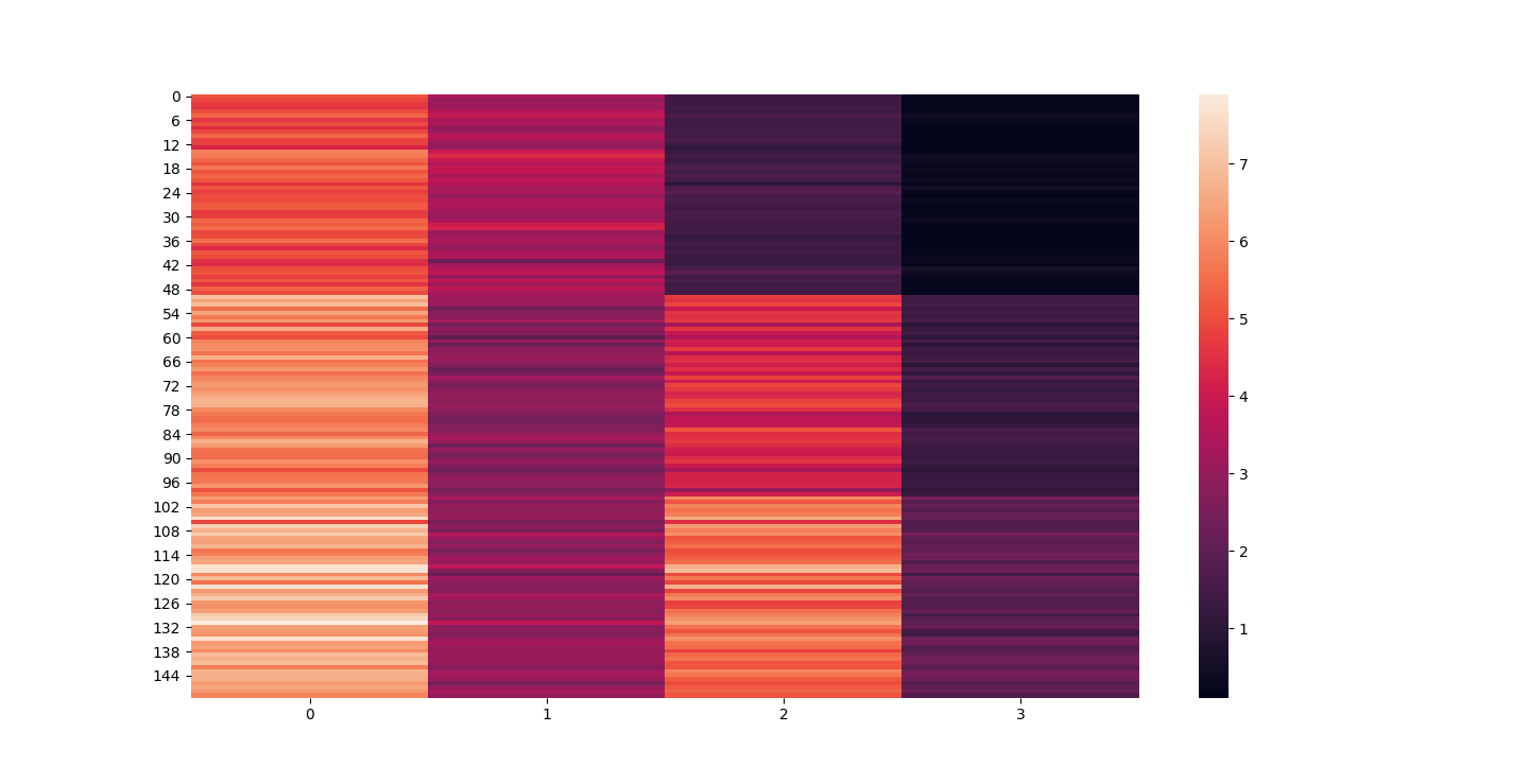
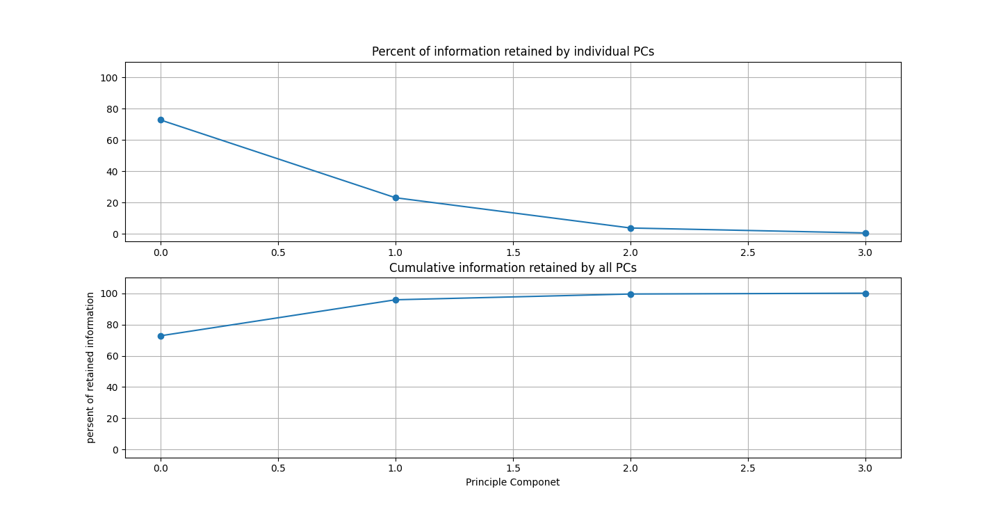
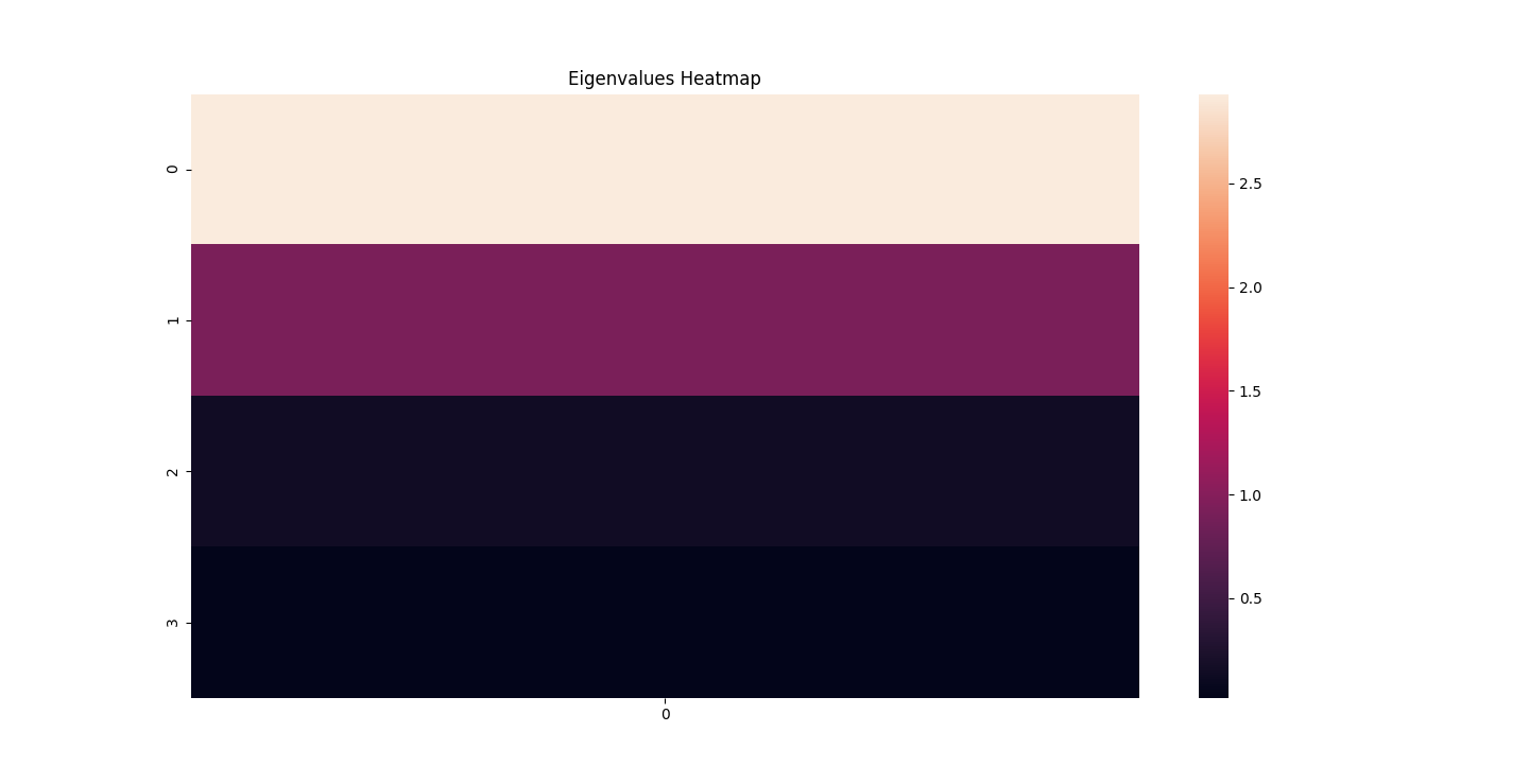
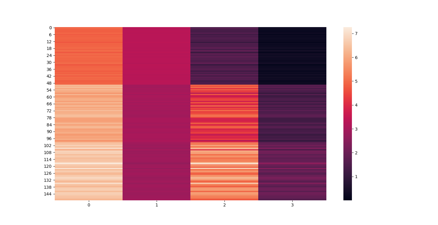
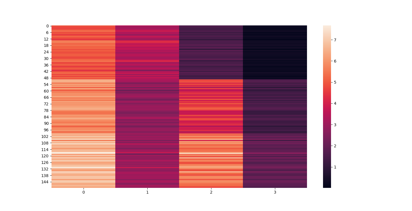
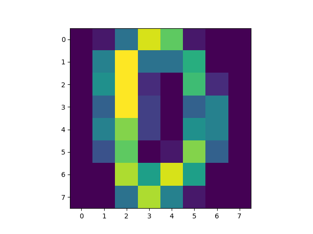
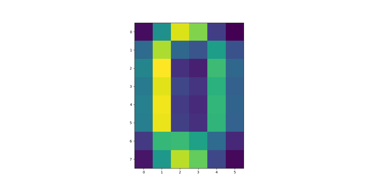
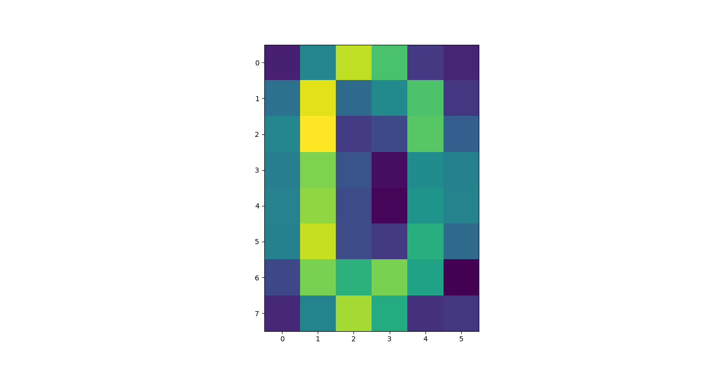
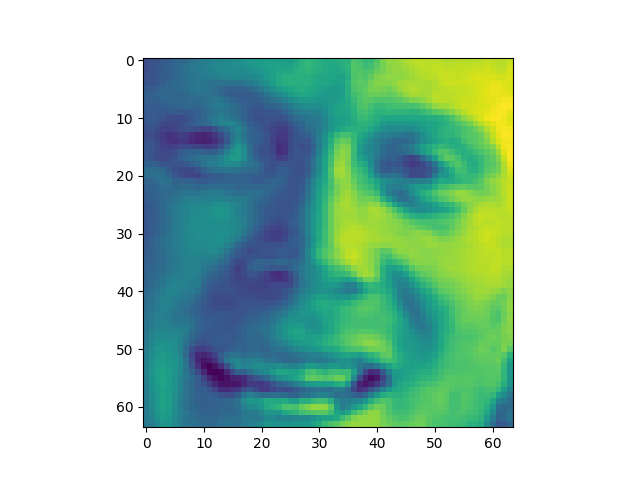
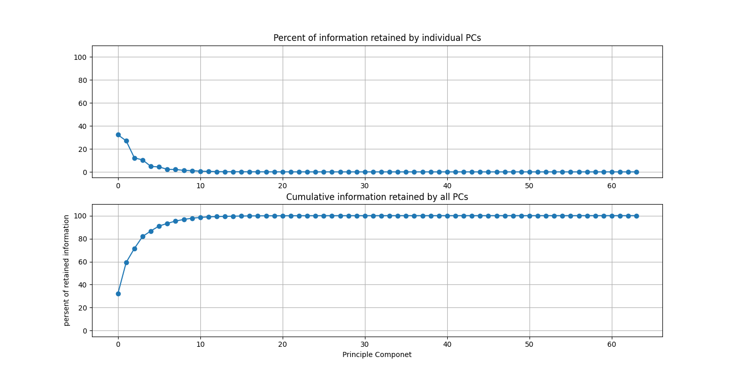
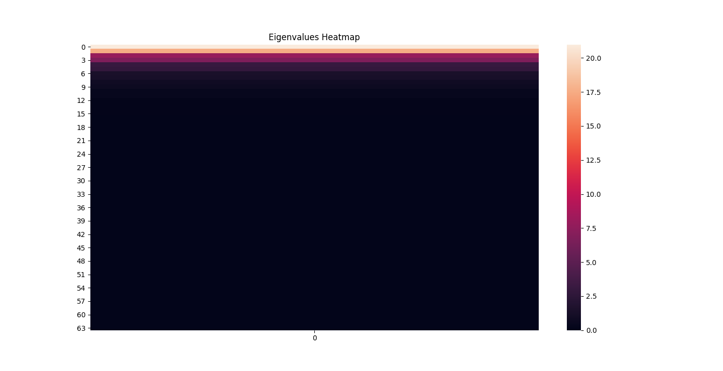
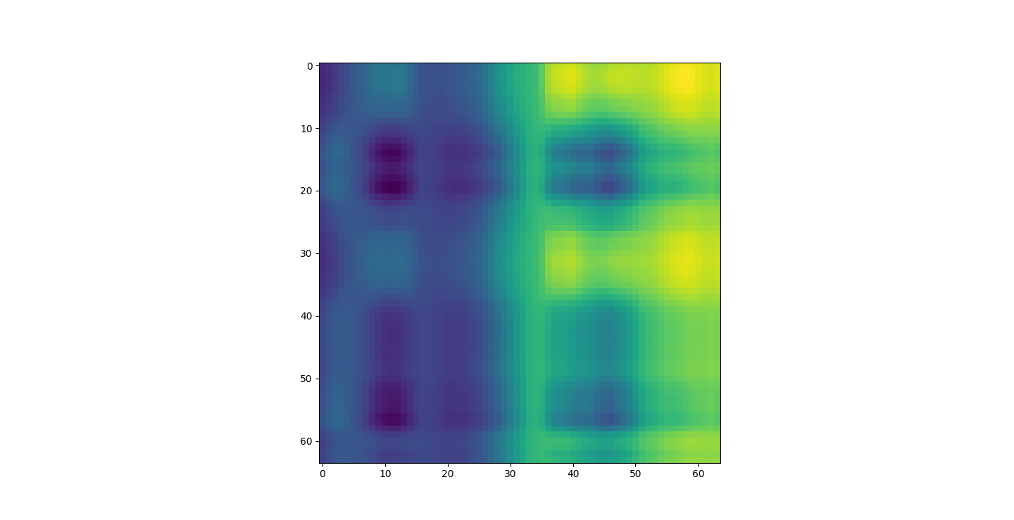
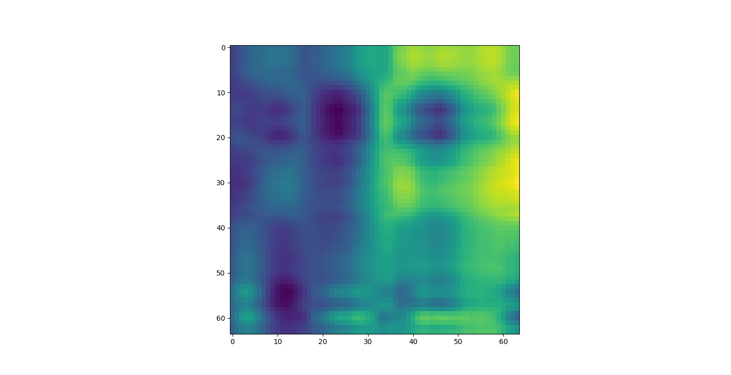
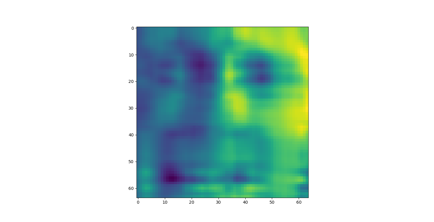
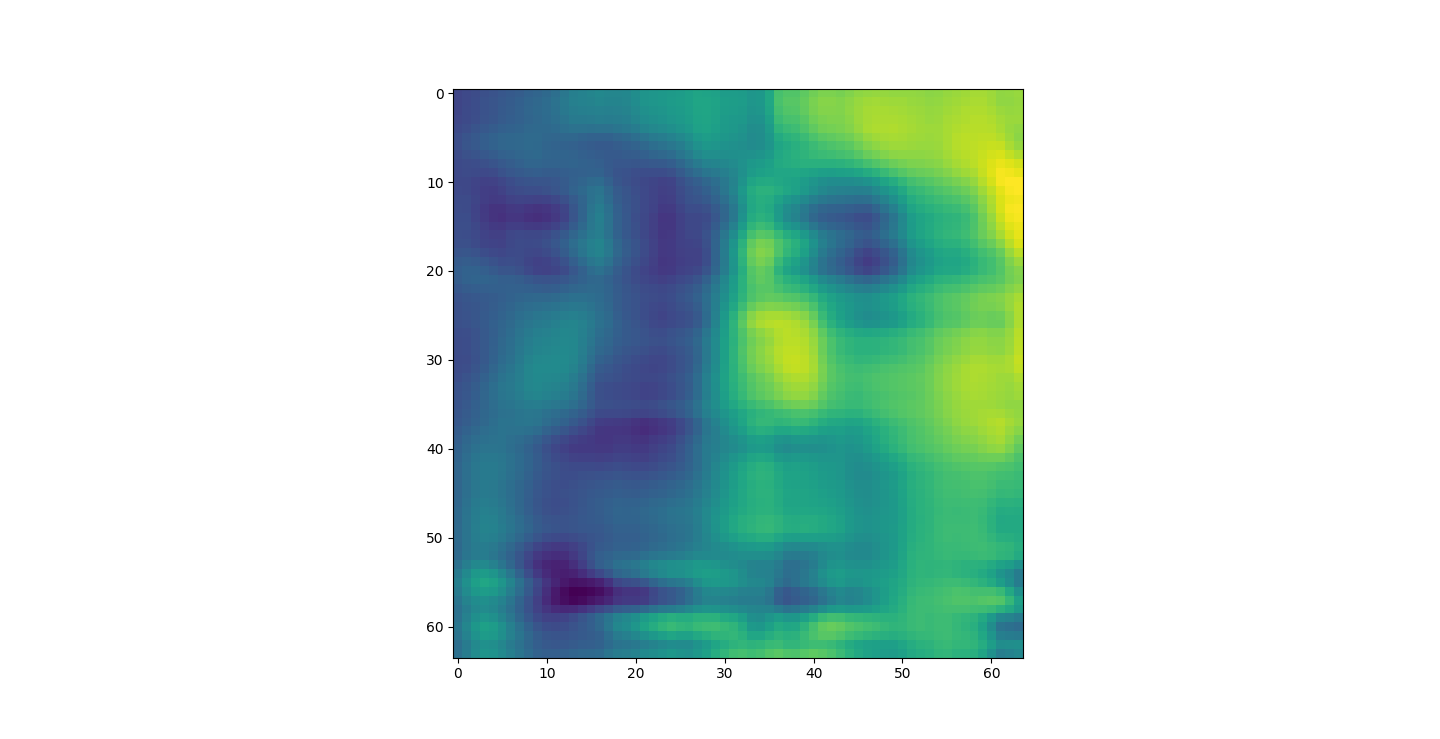
There are three parts to this report. Each part includes an eigenvector heatmap, a scaled eigenvector scree plot, and reconstructions of four stages of data retention. The Optdigits and LFW Crop sections include the showcase of random images alongside a data retention showcase.
Iris Raw - Blue
Iris 25% PCA - Red
For this graph I tried to use contrasting colors but I think red overtook blue. That and because blue holds more detail it might not be able to stand its ground visually against red 20% PCA.
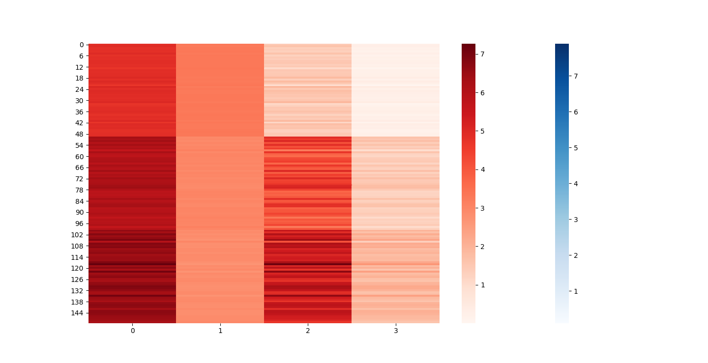
At d = 1 this holds 25% of our data. It clearly still hold enough to identify Irises.
Sample taken = 0
Sample taken = 0
The appearance of the reconstructions as we retain more dimensions sharpen. However, we might want to take advantage of this. For example in Iris the best looking set was the 20% or 1d. This is definitly not the case with the other datasets. LFW was unrecognizable bellow 80%.
I saved an 80% or 4D projection of the first sample. The size of lfwcrop is 433,553,536, bites or aroun 433MB. There are 13231 frames inside of lfwcrop. That's around 32768 bytes per frame. Our projection is only 2176 bytes. That's 6.64% the size! That's a huge reduction! We can see that lfwcrop has 64 dimensions but our projection at 80% data retention has just 4 dimensions! 4/64 just happens to be 6.25%. That's very close to our real world value. I suspect the difference between our theoretical value and the one we got is overhead from numpy and the .npy filetype.
GNU General Public License v3.0
