Super-node Concept
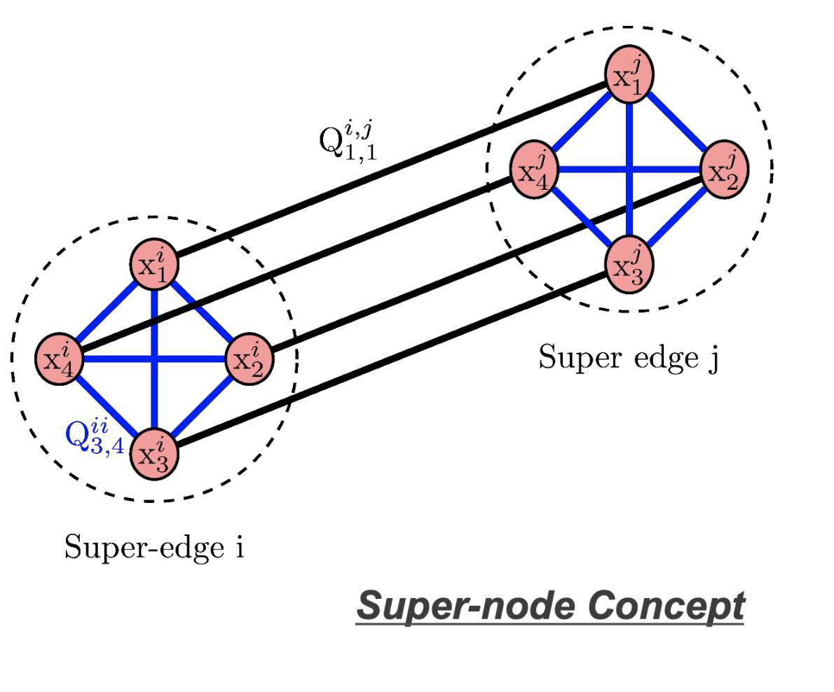
- Partition into
$k$ parts in parallel - Uses super-node concept
- Unary embedding
- k logical qubits per vertex
- New formulation requires a kn x kn QUBO
- Results in 1 of k qubits set on for each vertex
- Similar to graph coloring problem
- Useful for graph partitioning and community detection
| Constraint | Penalty Function |
|---|---|
| Concepts | Related terms |
|---|---|
| Binary Quadratic Models | BQM, Ising, QUBO |
| $\begin{array}{l}\text { Constrained Quadratic } \\text { Models }\end{array}$ | CQM, constrained quadratic model |
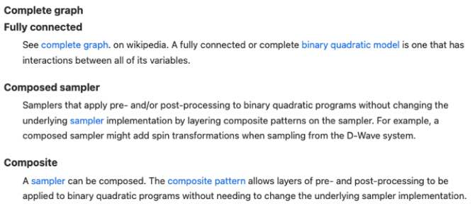
| Constraint Satisfaction | CSP, binary CSP |
| Discrete Quadratic Models | DQM, discrete quadratic model |
| Hybrid | quantum-classical hybrid, Leap's hybrid solvers, hybrid workflows |
| Minor-Embedding | $\begin{array}{l}\text { embedding, mapping logical variables to physical qubits, chains, chain } \\text { strength }\end{array}$ |
| Penalty Models | Penalty Models |
| Quadratic Models | Quadratic Models |
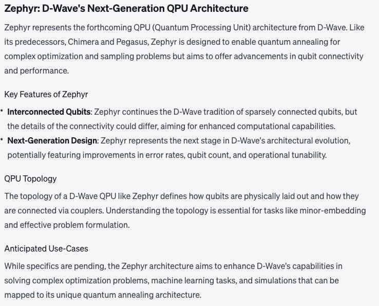
| QPU Topology | Chimera, Pegasus |
| Samplers and Composites | solver |
| Solutions | samples, sampleset, probabilistic, energy |
| Variables | binary, discrete, integer, real variables |
DiVincenzo's
electromagnetic wave propagating through a chain of identical qubits placed in a transmission line, and considered as an effective medium.
circuit formalism,
node
"flux"
time derivative
node potential (in CGS units)
CGS units
Lumped element circuit
ID quantum metamaterial:
chain of flux qubits
transmission line
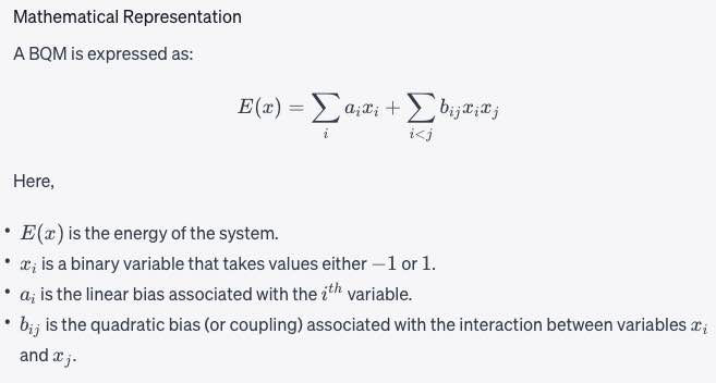
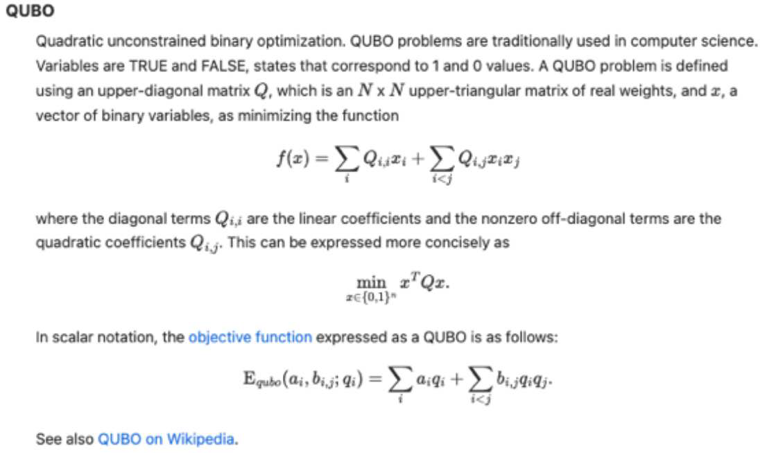
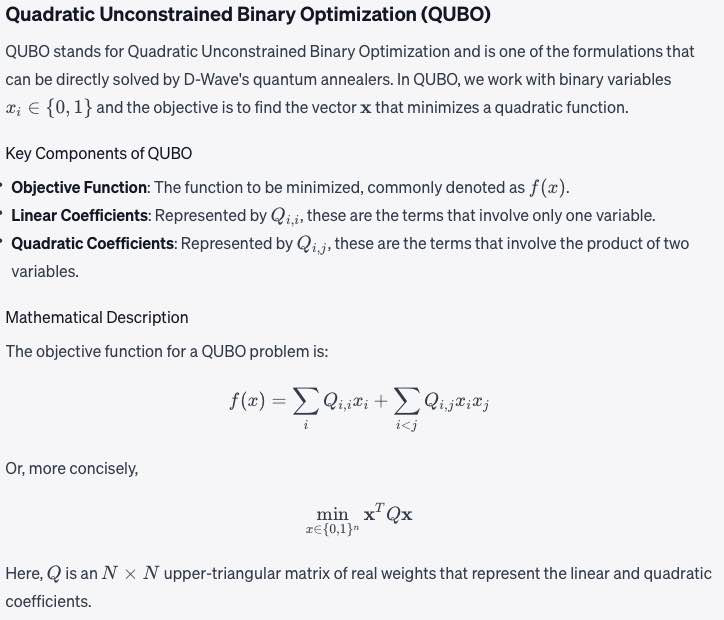
binary quadratic model
BQM
A collection of binary-valued variables (variables that can be assigned two values, for example
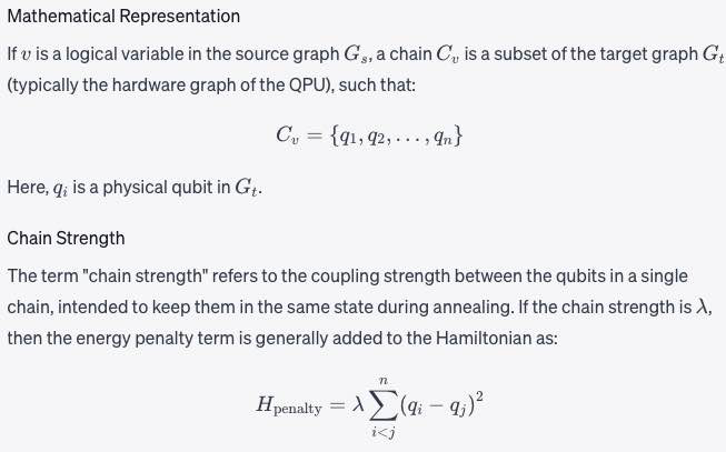
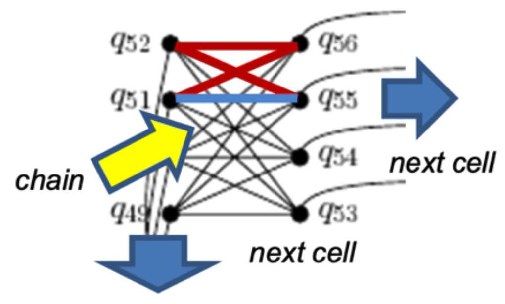
Chain One or more nodes or qubits in a target graph that represent a single variable in the source graph. See embedding. See a fuller description under Minor-Embedding.Chain and Minor-Embedding In the context of quantum computing, particularly with D-Wave systems, a chain refers to a collection of physical qubits on the quantum processing unit (QPU) that together represent a single logical variable from the problem being solved. Minor-embedding is the process of mapping these logical variables to these chains on the QPU.
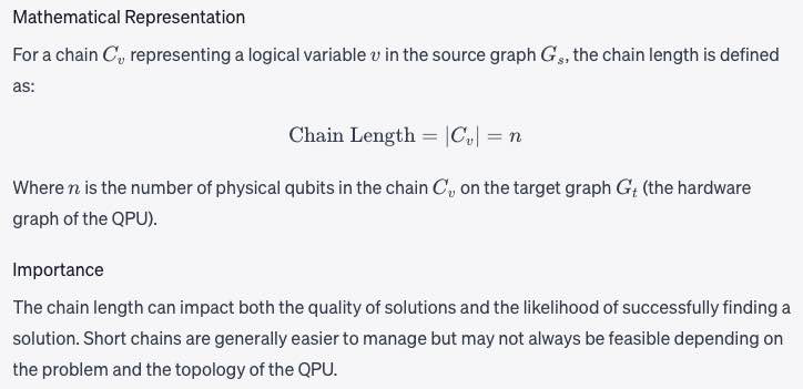
Chain length
The number of qubits in a Chain. See a fuller description under Minor-Embedding.Chain length refers to the number of physical qubits in a chain that represents a single logical variable in your problem formulation.
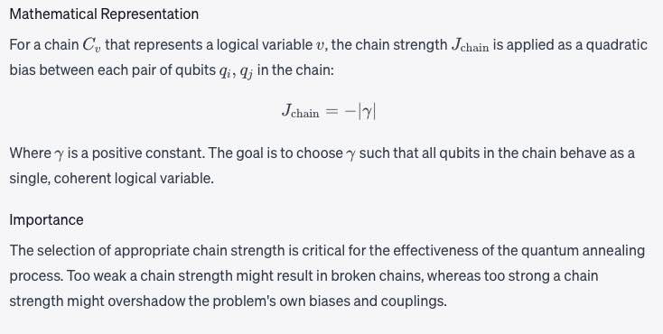
Chain strength
Magnitude of the negative quadratic bias applied between variables to form a chain. See a fuller description under Minor-Embedding. Chain strength refers to the magnitude of the negative quadratic bias applied between qubits in a chain to enforce that they take on the same value during the quantum annealing process.
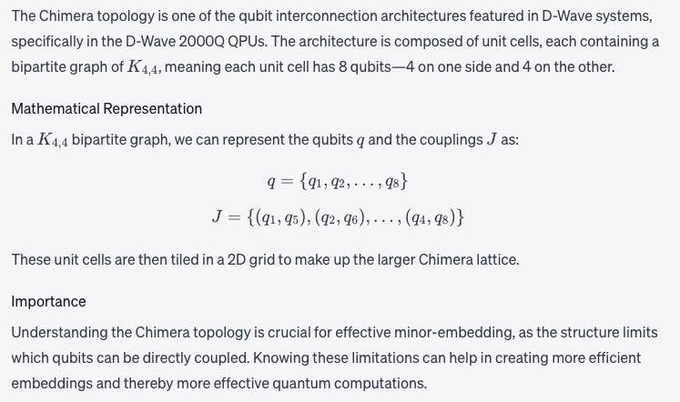
Chimera
A D-Wave QPU is a lattice of interconnected qubits. While some qubits connect to others via couplers, D-Wave QPUs are not fully connected. For D-Wave 2000Q QPUs, the qubits interconnect in an architecture known as Chimera. See a fuller description under QPU Topology. See also Pegasus and Zephyr. The Chimera topology is one of the qubit interconnection architectures featured in D-Wave systems, specifically in the D-Wave 2000 Q QPUs.
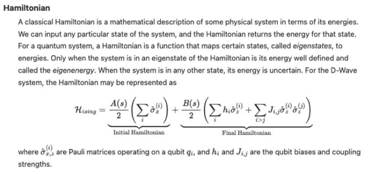
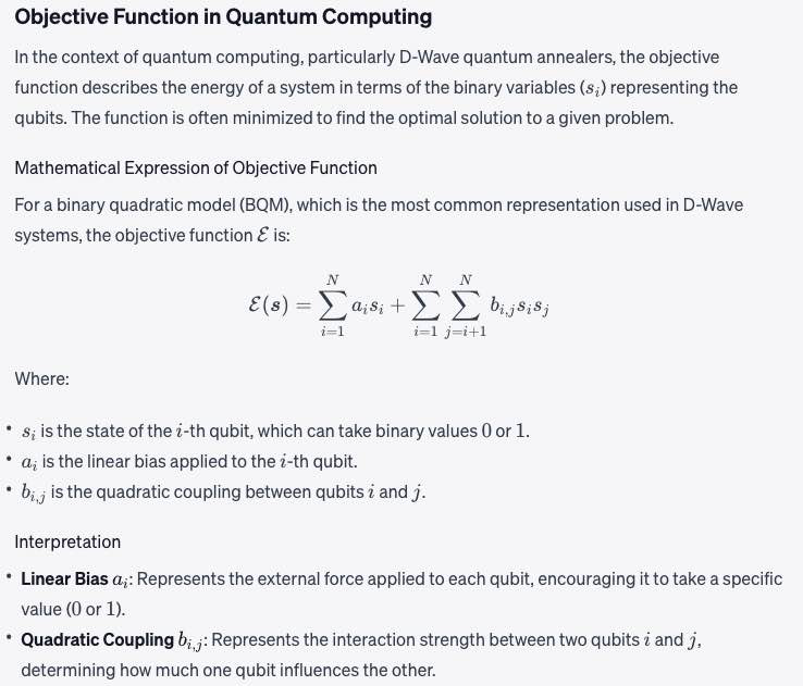
Objective function
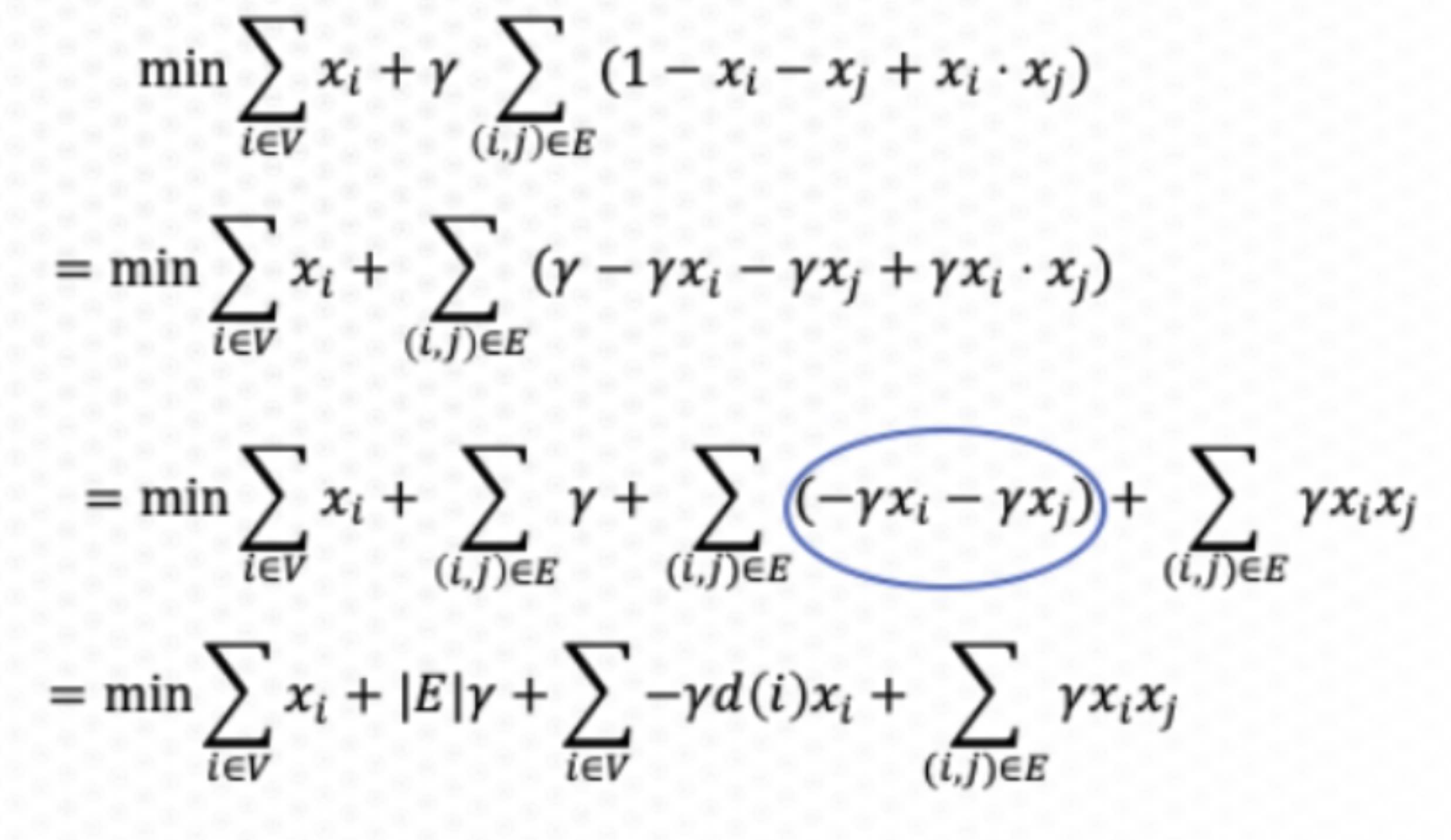
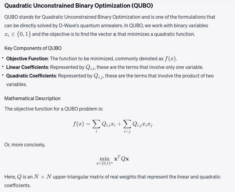
A mathematical expression of the energy of a system as a function of binary variables representing the qubits.
Math:
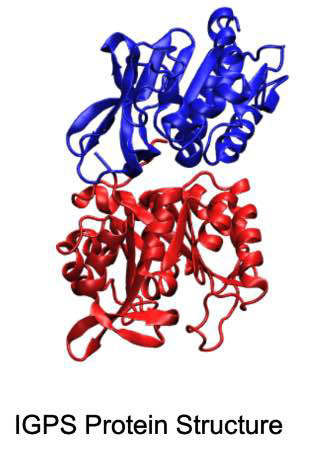
In this project, we explore the concept of community detection within bio-systems, with a specific focus on the enzyme IGPS found in bacteria. We use both classical algorithms such as Girvan-Newman and quantum algorithms using D-Wave's qbsolv to approach this optimization problem.
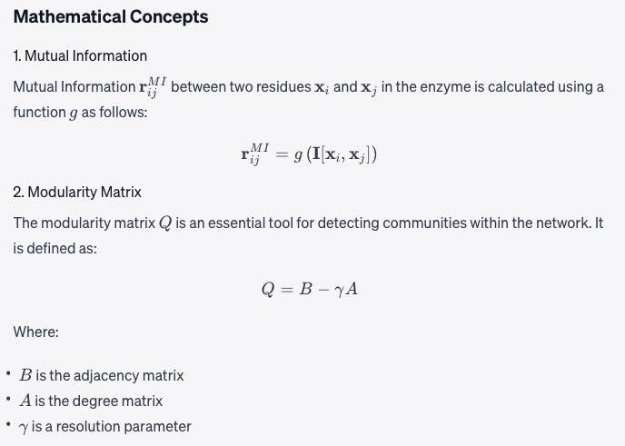
Mutual Information ( \mathbf{r}_{ij}^{MI} ) between two residues ( \mathbf{x}_i ) and ( \mathbf{x}_j ) in the enzyme is calculated using a function ( g ) as follows:
[ \mathbf{r}_{ij}^{MI} = g\left(\mathbf{I}[\mathbf{x}_i, \mathbf{x}_j]\right) ]
The modularity matrix ( Q ) is an essential tool for detecting communities within the network. It is defined as:
[ Q = B - \gamma A ]
Where:
- ( B ) is the adjacency matrix
- ( A ) is the degree matrix
- ( \gamma ) is a resolution parameter
To get started, install the required Python packages:
pip install numpy dwave-ocean-sdkHere's the Python3 code that demonstrates the community detection approach:
import numpy as np
from dwave.system import DWaveSampler, EmbeddingComposite
from dwave_qbsolv import QBSolv

# Generate a correlation matrix (This is a mock-up for demonstration)
n = 454  # Number of residues in IGPS
C = np.random.rand(n, n)

# Calculate modularity matrix
gamma = 1.0
A = np.sum(C, axis=0)
Q = C - gamma * np.outer(A, A) / np.sum(A)

# Prepare for qbsolv
Q_dict = {(i, j): Q[i, j] for i in range(n) for j in range(n)}

# Initialize D-Wave parameters
sampler = EmbeddingComposite(DWaveSampler())
response = QBSolv().sample_qubo(Q_dict, solver=sampler, num_repeats=10)

# Extract communities
best_sample = response.first.sample
communities = {node: state for node, state in best_sample.items()}The study aims to explore the computational efficacy of D-Wave in calculating structural balance in signed social networks. We conducted experiments on fully-connected graphs and compared the performance of D-Wave against a simulator.
- Topology Mismatch: Arbitrary networks often do not align with D-Wave's native topology, complicating the mapping process. Even simple structures like triangles pose challenges.
- Embedding Complexity: Creating the desired topology by chaining nodes together, a process called "embedding," is NP-hard.
- Hardware Limitations: Given the current D-Wave machine topology and available qubits, the upper limit for fully-connected, simulated nodes is approximately 49.
- Overhead Costs: A significant portion of the execution time on D-Wave is spent on communication and initialization, overshadowing the D-Wave's fast annealing time of 20 microseconds.
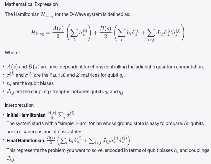
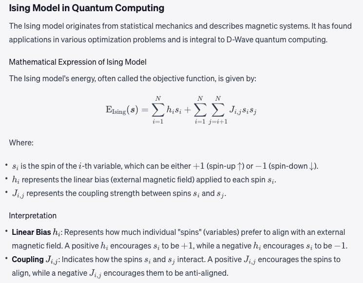
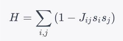
The Ising model equivalent to this problem is governed by the Hamiltonian:
[ H = \sum_{i, j} \left( 1 - J_{ij} s_i s_j \right) ]
Where ( J_{ij} ) and ( s_i ) are as described earlier.
Given the challenges, it's crucial to optimize the D-Wave code as much as possible. Here's a code snippet that minimizes overhead:
from dwave.system import DWaveSampler, EmbeddingComposite

# Predefined J matrix (mock example)
J = {(0, 1): 1, (1, 2): -1, (0, 2): -1}

# Initialize D-Wave sampler
sampler = DWaveSampler()
embedded_sampler = EmbeddingComposite(sampler)

# Sample with minimal overhead
params = {'num_reads': 1000, 'annealing_time': 20}  # Annealing time in microseconds
response = embedded_sampler.sample_ising({}, J, **params)

# Extract optimal assignment
best_sample = response.first.sample
optimal_assignment = {node: 'Positive' if state == 1 else 'Negative' for node, state in best_sample.items()}

print("Optimal Assignment:", optimal_assignment)
Citations /References:
Zagoskin, A. M. (2010). Why quantum engineering?. Low Temperature Physics, 36(10), 911-914. https://doi.org/10.1063/1.3515522
D-Wave Systems
Los Alomos National Lab
