R - second half.md

Quick Notes

• Parameter: a value that tells you something about a population
• Statistic: tells you something about a small part of the population
• Central limit theorem: when same size increase, sample mean will be normally distributed
• Quantitative: continuous, discrete, countable
• Qualitative: can't count, colours, soft/hard
• Parametric tests: are based on assumptions about the distribution of sample taken from population; most commonly assumes data is approximately normally distributed.
• Nonparametric tests: do not rely on assumptions about the shape or parameters of the underlying population distribution.
• R-squared: Coefficient of Determination is the measure of the variance in response variable ‘y’ that can be predicted using predictor variable ‘x’
• adjusted R-squared: penalizes for adding more variables to the model
• target variable: y
• Standard Deviation: quantifies the variation within a sect of measurements $\LARGE \text{SD}=\sqrt{\frac{\Sigma(x_i - \bar x)^2}{n-1}}$
• Standard Error: quantifies the variation in means from multiple sets of measurements
• Root Mean Square Error: $\LARGE \text{RMSE}=\sqrt{\frac{\Sigma(\text{Predicted}_i-\text {Actual}_i)^2}{N}}$
• log function = $\Large log (\frac{p}{1-p})$
• Logistic Regression
  • bias: the coefficients become unreliable
  • same old linear model, except the coefficients are log ratios
  • $\LARGE p=\frac{e^{log(odds)}}{1+e^{log(odds)}}$

Regression line: predicts the change in $y$ when $x$ increases by one unit.

• $\bar x$ = average of $x$
• $\bar y$ = average of $y$
• $r$ = cor() where $-1 \leq r^2 \leq 1 $ = measures the linear relationship between two quantitative variables with respect to direction and strength
• $s_x$ = sd()

PCA

• a type of linear transformation on a given data set that has values for a certain number of variables (coordinates) for a certain amount of spaces
• eigenvector is a direction; eigenvalue is a number telling you how much variance there is in the data in that direction
• eigenvector with the highest eigenvalue is, therefore, the first principal component
• works best with numerical data
• exclude categorical variables

R-squared or coefficient of determination

• $r^2$= r-squared where $0 \leq r^2 \leq 1$

  • measure how close each data point fits to the regression line
  • tells us how well regression line predicts actual values
  • the % of variation in $y$ that is account for by its regression on $x$
    • e.g. $r^2=0.88$ means 88% of the variation in $y-axis$ is account for by its regression on $x-axis$.

• $SS_{REGRESSION}$: the amount of variations exampled by using the regression equation

• $SS_{ERROR}$: the residual variation in the data that is not explained by independent variables

• $\Large SST_{\text{TOTAL}} = SSR_{\text{REGRESSION/EXPLAINED}} + SSE_{\text {ERROR/UNEXPLAINED}} $ $\LARGE R^2 = \frac{SSR_{EXPLAINED}}{SST_{TOTAL}} $ = variability explained by the regression / total variability of the dataset

  

$\LARGE SE_{line} = (y_1 - (mx_1 +b))^2 + (y_2 - (mx_2+b))^2 \dots + (y_n - (mx_n+b))^2 $

$\LARGE \text {total variation of } y = (y_1 - \bar y)^2 + (y_2 - \bar y)^2 \dots + (y_n - \bar y)^2 = SE_{\bar y}$

What % of total variation is not described by the regression line $\LARGE \text{Percentage not described by regression line}= \frac{SE_{line}}{SE_{\bar y}}=\frac{SSE}{SST}$

What % described by regression line; The coefficient determination? small = good fit $\LARGE \text{Percentage described by regression line}= R^2 = 1-\frac{SE_{line}}{SE_{\bar y}}=\frac{SSR}{SST}$

Explanation

$SE_{line}$ is small = line is good fit = $r^2$ close to $1$

$SE_{line}$ is large = 1 minus will make it close to 0 = $r^2$ close to $0$

Dimensionality Reduction

7 ways to clean data

1. Removing data columns with too many miss values; remove columns with NAs

   • missing data rate = # missing values / total # of rows

2. Remove column with low variance

   • check how far away from the average

   • normalize to [0,1], then calculate each column variance and remove columns with a variance below a given threshold.

3. Reduce Highly Correlated Columns/variables/attributes

   • measure correlation between pairs of column
   • remove highly correlated data column without decreasing the amount of information dramatically
     • filter
     • wrapper
     • hybrid

4. PCA (feature extraction)

   • a stat procedure using orthogonal transformation to move original n coordinates of a dataset to new set of n coordinate
   • purpose to reduce dimensionality by finding a new smaller set of m variables, m < n, retaining most of the data information
   • sensitive to the relative scaling; normalized before applying PCA
   • data set loses its interpretability, otherwise PCA is not for your project
   • if $z_1+z_2+z_3$ explains 98% of the variation, then can consider scope out the remaining

5. Tree Ensembles - Random Forest (feature selection), Logistic Regression, any model

   • RF
     • boot strapped dataset; with replacement

6. Backward Feature Elimination

7. Forward Feature Construction

Dimensionality Reduction

• Reason: curse of dimensionality.

  • Two families
    • Feature Selection; Random Forest
      • effective to pick good features, from $x_n$ to $x_m$ where $n &gt; m$
      • ending result is a subset
      • pros: interpretability; can still interpret the model e.g. is the age still relevant?
      • cons: bad performance
    • Feature Extraction; PCA
      • transform $x_n$ to $z_m$ where $n \geq m$
      • converts the dimension; changes labels.
      • pros: high performance; high variance on the first few columns
      • cons: no interpretability; working in another dimension

• Remove data columns with too many missing values;

• Low variance filter

• Reducing highly correlated columns

Principal Component Analysis (PCA)

• scale = false - finding the min and max of a column and then scale it. Use for normalization.
• centre = false - shifting the date to the origin
• creating different PC
• each PC*(each feature)

Dimensionality reduction via random forest

• effective to pick good features

Feature selection

• Caret package - very effective package

Principal Component Analysis (PCA)

• to minimize dimensions; transform data technique
• transform to less than or equal
• no loss of info
• converts the correlation (or lack there of)
• the axis are rank in order of importance. PC1, PC2, ...
• R command princomp
• usually choose PC with SD over 1.
• using loadings to get the coefficients

Statistical Learning Methods

Classification

• predictive method; predicting categorical variable; predict the class
• divide data to train/test
• supervised
  • ML task of interring a function from labelled training data.
• two different classifications
  • binary classification - T/F
  • multi-class classification - assigning object to one of several

Logistic regression

Naïve Bayes classifier

$k$-fold cross-validation

• divide into to $k$ chunks.
• take one chunk out as test and rest as training
• do so $k$ times, each time with a new chunk out
• average result from $k$ experiments

Decision trees

Lecture example

$k$-Nearest Neighbours (kNN)

• train/test
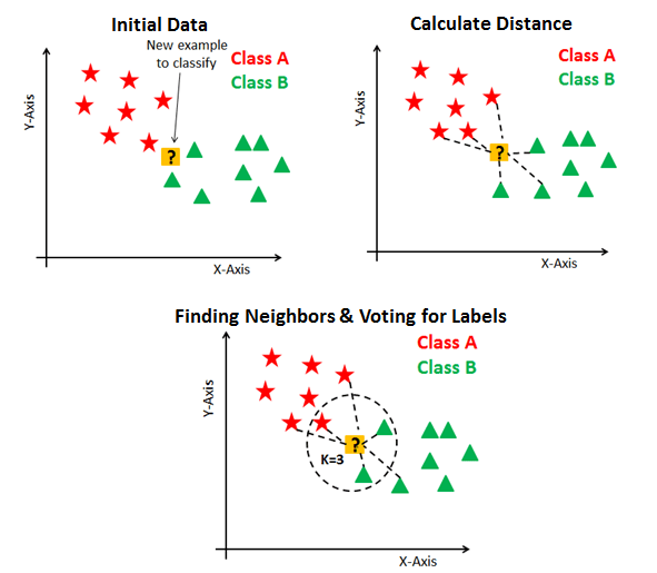
• mostly used in pattern recognition
• draw a circle until it has $k$ neighbours, majority rules
• $k$ = odd number to avoid draws.
• using distance function
• • Euclidean, Manhattan, Makowski
• feature should be on same scale
• can be use for both
• • classification - uses majority rule
  • regression - takes average
• compute test point distances for every training point

Lecture example

Random Forest (RF)

• built from decision trees
• steps
  1. create bootstrap data by randomly sample; can be repeated
  2. create a decision tree with this bootstrap data of n rows
  3. randomly select 2 columns for the root node
     1. out of the two find the highest entropy
  4. repeat #3
  5. repeat #2 x100
• how to use
  1. we get new data, and run it on first tree
  2. keep track of the results
  3. go back to #1 using second tree
  4. after finishing all trees, we see which has the most votes
• estimate the accuracy of the RF
  1. using new data, we run it on out-of-boot trees
  2. record result; repeat until no more trees
  3. tally the result
  4. repeat for all out-of-bag samples, for all trees
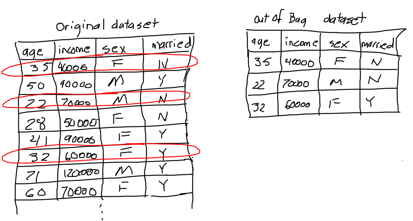
• typically 1/3 of the data didn't end up in bootstrap data.
• bagging: bootstrapping data plus using aggregate to make a decision
• Out-Of-Bag dataset: the entries that didn't make it to the bootstrap
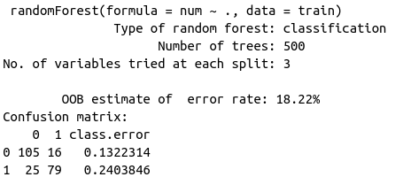
• Goals
  • measure the accuracy of our random forest
    • by the proportion of Out-Of-Bag samples that were correctly classified by the RF
• out-of-bag error: proportion of out-of-bag samples that were incorrectly classified
• for each variable
  • mean decrease accuracy
    • measures the predictive accuracy of the resulting tree
  • mean decrease impurity
    • how many times it has been selected in a split
    • measure of the variable split where the split gives the lowest Gini index (lower = purer/better)
      • Gini Impurity reaches zero when all records in a group fall into a single category
    • Mean Decrease in Gini is the average (mean) of a variable’s total decrease in node impurity, weighted by the proportion of samples reaching that node in each individual decision tree in the random forest. This is effectively a measure of how important a variable is for estimating the value of the target variable across all of the trees that make up the forest. A higher Mean Decrease in Gini indicates higher variable importance.
• more comparisons
  • previously used 2 columns
  • then we compare with 3 columns and see which yields the best results
  • typically choose square root of # of variables.

Clustering

• descriptive method; exploring dataset; getting descriptions; no predictions
• tasks of grouping objects, so the group are more similar than others
• unsupervised
  • ML tasks inferring function to describe hidden structure of unlabelled data.
• two types
  • Centroid-based clustering
    • divided to non-overlapping cluster
  • Hierarchical clustering
    • nested clusters organized as a hierarchical tree
    • tells you: what two things are most similar

$k$-means clustering (k-means)

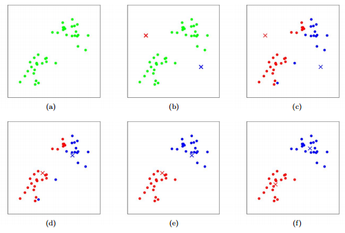
• each has a centroid (centre point); doesn't have to be a member of the dataset
• $k$ = number of clusters
• randomize k different initial means;

How it works?

1. randomly assign k centroids
2. find all points that's closest to the centroid
3. calculate the mean of x and y of all the dots in the same group
4. move centroid to that mean
5. repeat #2

Lecture example

Regression

4 Assumptions

1. Linearity/Correct functional form: The relationship between X and the mean of Y is linear.

   • linear in the parameters; cannot have like $x^2$
   • have an additive regression

2. Homoscedasticity/Constant Error variance: The variance of residual is the same for any value of X.

   • i.e. the distance between the dot and the regression line, the variance should be about the same as x increases
   • if x is low, the variance is so big; if the x is high, the variance is also so big
   • remedy: can log things

3. Independence: Observations are independent of each other.

   • precedent has an effect on the current.

4. Normality: For any fixed value of X, Y is normally distributed.

Understanding R results in lm()

1. Std. Error is the standard deviation of the sampling distribution of the estimate of the coefficient under the standard regression assumptions. Such standard deviations are called standard errors of the corresponding quantity (the coefficient estimate in this case).

   In the case of simple regression, it's usually denoted sβ^sβ^, as here. Also see this

   For multiple regression, it's a little more complicated, but if you don't know what these things are it's probably best to understand them in the context of simple regression first.

2. t value is the value of the t-statistic for testing whether the corresponding regression coefficient is different from 0.

   The formula for computing it is given at the first link above.

3. Pr. is the p-value for the hypothesis test for which the t value is the test statistic. It tells you the probability of a test statistic at least as unusual as the one you obtained, if the null hypothesis were true. In this case, the null hypothesis is that the true coefficient is zero; if that probability is low, it's suggesting that it would be rare to get a result as unusual as this if the coefficient were really zero.

Linear regression

• aim: to minimize the error
  • least squares
  • minimize the sum square residuals
• assumes
  • the input/output variable are linear
• quick note:
  • sum up square residuals (distance: dot to line)
  • variance: average SS per dot
• recommended
  • normalization independent variable
  • remove outliers
  • remove highly correlated variables to reduce overfitting
  • check distribution of errors; errors should be normally distributed
• simple linear regression
  • 1 dependent, 1 independent
• multiple linear regression
  • 1 dependent, multiple independent

Equation $$ \LARGE y=\beta_0+\beta_1x_1+\beta_2x_2+\dots+\beta_1k_k+\epsilon $$

• $\LARGE y$ = response variable
• $\LARGE \beta_0,\beta_1,\beta_2,\dots\beta_k$ = unknown constants; coefficients
• $\LARGE x_1,x_2,\dots x_k$ = predictor variables
• $\LARGE \epsilon$ = random error

Logistic regression

• types
  • binomial logistic regression
    • 2 dependent variables
  • multinomial logistic regression
    • more than 2 dependent
• aim:
  • predict possibilities of outcome of categorical dependent variable
• independent variable can have many
• logistic regression is a linear model; despite using the $log(odds)$
• can be used as a regression, or classifier
• logistic is a linear algorithm
• sample size:
  • $N \geq 50+8k \text{ where k = independent variables; N=observations}$

Read chapter 13.

logistic regression or logit regression or logit model

Formula

dependent variable is categorical $$ \Large f(x)=\frac{1}{1+e^{-x}}\ P(A)+P(B)=1 $$

Transforming Linear to Logistic $$ \LARGE \frac{e^{ax+b}}{1+e^{ax+b}}=p\ \LARGE e^{ax+b}=p+pe^{ax+b}\ \LARGE e^{ax+b}-pe^{ax+b}=p\ \LARGE (1-p)e^{ax+b}=p\ \LARGE e^{ax+b}=\frac{p}{1-p}\ \LARGE log(e^{ax+b}) = log(\frac{p}{1-p})\ \LARGE ax+b=log(\frac{p}{1-p})=\text{logit p}\ \Large \text {x: independent variable}\ \Large \text {y: probability} $$ logistic regression = linear regression on the logit transform of $y$, where $y$ is the probability of success at each value of $x$.

Regression trees

• when used for regression
• as oppose to decision tree used for categorical dependent variable; regression tree when response either discrete or continuous.

Variable Selection for Regression

• important: deal with outliers first

Forward Selection

• begin with no variables
• then pick first independent variable with highest R-square
  • number that indicates the proportion of variance in dependent variable for a specific independent variable
    • $R^2 = 1$ ... it explains all variations
    • $R^2 = 0$ ... it explains none
  • pick the next which increases the R-square the most
• similar to adjusted R-square, penalizes for adding variables
• only compare AIC value whether its increasing or decreasing by adding more variables
• lower AIC is preferred

Backward Elimination

• start with all variables
• remove variable with least significant

Stepwise regression

• a combo of forward and backward
• after adding, all other remaining variables are checked
• need to decide on:
  • significant level for adding
  • significant level for remove

Akaike Info Criterion (AIC)

$f(DF,MSE)$

starting with the y-intercept; with addition; minimizing the AIC

Notice

1. be careful comparing AIC value between different packages
2. AIC is a in-sample measure. Can only compute the AIC values using the training set
3. not a measure of prediction (accuracy)

Bayesian Info Criterion BIC

$f(DF,MSE,N)$ where $N = \text {number of observations}$

Plain images

$R^2$

Standard Deviation vs Standard Error

Random Forest

Cross-Validation

Confusion Matrix